Chapter 9 Data Transformation
9.1 Introduction to Data
The upcoming weeks will be focused on using R for data cleaning and analysis. Let’s first get on the same page with some terms:
A variable is a quantity, quality, or property that you can measure.
An observation is a set of measurements for the same unit. An observation will contain several values, each associated with a different variable. I will sometimes refer to an observation as a data point or an element.
A value is the state of a variable for a particular observation.
Tabular data are a set of values, each associated with a variable and an observation. Tabular data have rows (observations) and columns (variables). Tabular data are also called rectangular data or spreadsheets.
9.1.1 The Gapminder Dataset
This lesson discusses how to perform basic exploratory data analysis.
For this unit, we will be working with the “Gapminder” dataset, which is an excerpt of the data available at gapminder.org. For each of 142 countries, the data provide values for life expectancy, GDP per capita, and population, every five years from 1952 to 2007.
9.1.2 Structure and Dimensions
By loading the gapminder package, we now have access to a data frame by the same name. Get an overview of this with str(), which displays the structure of an object.
str(gap)
#> tibble [1,704 × 6] (S3: tbl_df/tbl/data.frame)
#>  $ country  : Factor w/ 142 levels "Afghanistan",..: 1 1 1 1 1 1 1 1 1 1 ...
#>  $ continent: Factor w/ 5 levels "Africa","Americas",..: 3 3 3 3 3 3 3 3 3 3 ...
#>  $ year     : int [1:1704] 1952 1957 1962 1967 1972 1977 1982 1987 1992 1997 ...
#>  $ lifeExp  : num [1:1704] 28.8 30.3 32 34 36.1 ...
#>  $ pop      : int [1:1704] 8425333 9240934 10267083 11537966 13079460 14880372 12881816 13867957 16317921 22227415 ...
#>  $ gdpPercap: num [1:1704] 779 821 853 836 740 ...
str() will provide a sensible description of almost anything and, worst case, nothing bad can actually happen. When in doubt, just str() some of the recently created objects to get some ideas about what to do next.
We could print the gapminder object itself to screen. However, if you have used R before, you might be reluctant to do this, because large datasets just fill up your Console and provide very little insight.
The head function displays the first 6 rows of any dataframe.
head(gap)
#> # A tibble: 6 x 6
#>   country     continent  year lifeExp      pop gdpPercap
#>   <fct>       <fct>     <int>   <dbl>    <int>     <dbl>
#> 1 Afghanistan Asia       1952    28.8  8425333      779.
#> 2 Afghanistan Asia       1957    30.3  9240934      821.
#> 3 Afghanistan Asia       1962    32.0 10267083      853.
#> 4 Afghanistan Asia       1967    34.0 11537966      836.
#> 5 Afghanistan Asia       1972    36.1 13079460      740.
#> 6 Afghanistan Asia       1977    38.4 14880372      786.
Here are some more common ways to query info from a dataframe:
# Get number of rows and columns:
dim(gap)
#> [1] 1704    6

# See column names:
names(gap)
#> [1] "country"   "continent" "year"      "lifeExp"   "pop"       "gdpPercap"

# A statistical overview can be obtained with summary():
summary(gap)
#>         country        continent        year         lifeExp
#>  Afghanistan:  12   Africa  :624   Min.   :1952   Min.   :23.6
#>  Albania    :  12   Americas:300   1st Qu.:1966   1st Qu.:48.2
#>  Algeria    :  12   Asia    :396   Median :1980   Median :60.7
#>  Angola     :  12   Europe  :360   Mean   :1980   Mean   :59.5
#>  Argentina  :  12   Oceania : 24   3rd Qu.:1993   3rd Qu.:70.8
#>  Australia  :  12                  Max.   :2007   Max.   :82.6
#>  (Other)    :1632
#>       pop             gdpPercap
#>  Min.   :6.00e+04   Min.   :   241
#>  1st Qu.:2.79e+06   1st Qu.:  1202
#>  Median :7.02e+06   Median :  3532
#>  Mean   :2.96e+07   Mean   :  7215
#>  3rd Qu.:1.96e+07   3rd Qu.:  9325
#>  Max.   :1.32e+09   Max.   :113523
#>
9.1.3 Variables
To specify a single variable from a data frame, use the dollar sign $. Let’s explore the numeric variable for life expectancy.
head(gap$lifeExp)
#> [1] 28.8 30.3 32.0 34.0 36.1 38.4
summary(gap$lifeExp)
#>    Min. 1st Qu.  Median    Mean 3rd Qu.    Max.
#>    23.6    48.2    60.7    59.5    70.8    82.6
hist(gap$lifeExp)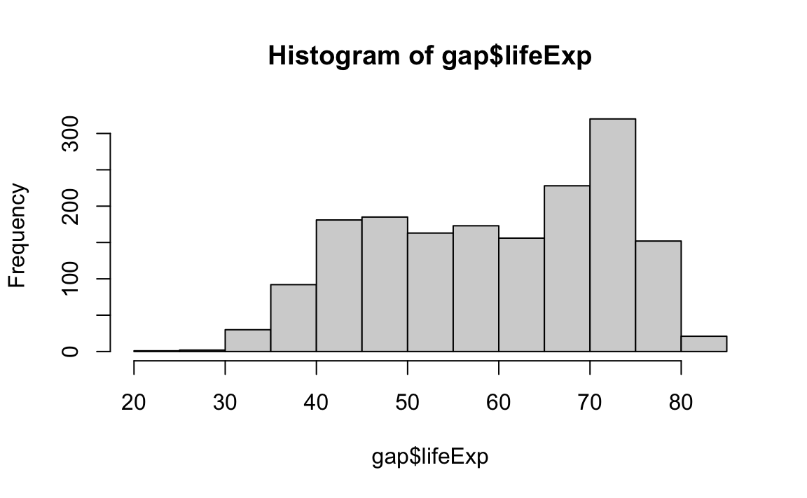
Data frames – unlike matrices in R – can hold variables of different flavors, such as character data (subject ID or name), quantitative data (white blood cell count), and categorical information (treated vs. untreated).
For example, the year variables is numeric, while the variables for country and continent hold categorical information, which is stored as a factor in R.
summary(gap$year)
#>    Min. 1st Qu.  Median    Mean 3rd Qu.    Max.
#>    1952    1966    1980    1980    1993    2007
summary(gap$country)
#>              Afghanistan                  Albania                  Algeria
#>                       12                       12                       12
#>                   Angola                Argentina                Australia
#>                       12                       12                       12
#>                  Austria                  Bahrain               Bangladesh
#>                       12                       12                       12
#>                  Belgium                    Benin                  Bolivia
#>                       12                       12                       12
#>   Bosnia and Herzegovina                 Botswana                   Brazil
#>                       12                       12                       12
#>                 Bulgaria             Burkina Faso                  Burundi
#>                       12                       12                       12
#>                 Cambodia                 Cameroon                   Canada
#>                       12                       12                       12
#> Central African Republic                     Chad                    Chile
#>                       12                       12                       12
#>                    China                 Colombia                  Comoros
#>                       12                       12                       12
#>         Congo, Dem. Rep.              Congo, Rep.               Costa Rica
#>                       12                       12                       12
#>            Cote d'Ivoire                  Croatia                     Cuba
#>                       12                       12                       12
#>           Czech Republic                  Denmark                 Djibouti
#>                       12                       12                       12
#>       Dominican Republic                  Ecuador                    Egypt
#>                       12                       12                       12
#>              El Salvador        Equatorial Guinea                  Eritrea
#>                       12                       12                       12
#>                 Ethiopia                  Finland                   France
#>                       12                       12                       12
#>                    Gabon                   Gambia                  Germany
#>                       12                       12                       12
#>                    Ghana                   Greece                Guatemala
#>                       12                       12                       12
#>                   Guinea            Guinea-Bissau                    Haiti
#>                       12                       12                       12
#>                 Honduras         Hong Kong, China                  Hungary
#>                       12                       12                       12
#>                  Iceland                    India                Indonesia
#>                       12                       12                       12
#>                     Iran                     Iraq                  Ireland
#>                       12                       12                       12
#>                   Israel                    Italy                  Jamaica
#>                       12                       12                       12
#>                    Japan                   Jordan                    Kenya
#>                       12                       12                       12
#>         Korea, Dem. Rep.              Korea, Rep.                   Kuwait
#>                       12                       12                       12
#>                  Lebanon                  Lesotho                  Liberia
#>                       12                       12                       12
#>                    Libya               Madagascar                   Malawi
#>                       12                       12                       12
#>                 Malaysia                     Mali               Mauritania
#>                       12                       12                       12
#>                Mauritius                   Mexico                 Mongolia
#>                       12                       12                       12
#>               Montenegro                  Morocco               Mozambique
#>                       12                       12                       12
#>                  Myanmar                  Namibia                    Nepal
#>                       12                       12                       12
#>              Netherlands              New Zealand                Nicaragua
#>                       12                       12                       12
#>                    Niger                  Nigeria                   Norway
#>                       12                       12                       12
#>                     Oman                 Pakistan                   Panama
#>                       12                       12                       12
#>                  (Other)
#>                      516
summary(gap$contintent)
#> Warning: Unknown or uninitialised column: `contintent`.
#> Length  Class   Mode
#>      0   NULL   NULL
Sometimes we need to do some basic checking for the number of observations or types of observations in our dataset. To do this quickly and easily, table() is our friend.
Let’s look at the number of observations first by region, and then by both region and year:
table(gap$continent)
#>
#>   Africa Americas     Asia   Europe  Oceania
#>      624      300      396      360       24
table(gap$continent, gap$year)
#>
#>            1952 1957 1962 1967 1972 1977 1982 1987 1992 1997 2002 2007
#>   Africa     52   52   52   52   52   52   52   52   52   52   52   52
#>   Americas   25   25   25   25   25   25   25   25   25   25   25   25
#>   Asia       33   33   33   33   33   33   33   33   33   33   33   33
#>   Europe     30   30   30   30   30   30   30   30   30   30   30   30
#>   Oceania     2    2    2    2    2    2    2    2    2    2    2    2
We can even divide by the total number of rows to get proportion, percent, etc.:
9.1.4 Challenges
Challenge 1.
Read the polity_sub dataset in the Data sub-directory.
Challenge 2.
Report the number and name of each variable in the dataset.
Challenge 3.
What is the mean polity2 score in the dataset?
Challenge 4.
What is the range of the polity2 variable?
Challenge 5.
How many unique countries are in the dataset?
9.2 Introduction to dplyr
9.2.1 tidyverse
It is often said that 80% of data analysis is spent on the process of cleaning and preparing the data.
Dasu and Johnson, 2003
For most applied researchers, data preparation usually involves 3 main steps:
- Transforming data frames, e.g., filtering, summarizing, and conducting calculations across groups.
- Tidying data into the appropriate format.
- Merging or linking several datasets to create a bigger dataset.
The tidyverse is a suite of packages designed specifically to help with these steps. These are by no means the only packages out there for data wrangling, but they are increasingly popular for their readable, straightforward syntax and sensible default behaviors.
In this chapter, we are going to focus on how to use the dplyr package for data transformation tasks.
For this unit, we will be working with the Gapminder dataset again.
library(tidyverse)
library(gapminder)

gap <- gapminder
head(gap)
#> # A tibble: 6 x 6
#>   country     continent  year lifeExp      pop gdpPercap
#>   <fct>       <fct>     <int>   <dbl>    <int>     <dbl>
#> 1 Afghanistan Asia       1952    28.8  8425333      779.
#> 2 Afghanistan Asia       1957    30.3  9240934      821.
#> 3 Afghanistan Asia       1962    32.0 10267083      853.
#> 4 Afghanistan Asia       1967    34.0 11537966      836.
#> 5 Afghanistan Asia       1972    36.1 13079460      740.
#> 6 Afghanistan Asia       1977    38.4 14880372      786.
9.2.2 Why dplyr?
If you have ever used base R before, you know the following will calculate the mean GDP per capita within each region:
mean(gap$gdpPercap[gap$continent == "Africa"])
#> [1] 2194
mean(gap$gdpPercap[gap$continent == "Americas"])
#> [1] 7136
mean(gap$gdpPercap[gap$continent == "Asia"])
#> [1] 7902
But this is not ideal because it involves a fair bit of repetition. Repeating yourself will cost you time, both now and later, and potentially introduce some nasty bugs.
Luckily, the dplyr package provides a number of very useful functions for manipulating dataframes. These functions will save you time by reducing repetition. As an added bonus, you might even find the dplyr grammar easier to read.
Here, we are going to cover 7 of the most commonly used dplyr functions. We will also cover pipes (%>%), which are used to combine those functions.
select()filter()mutate()arrange()count()group_by()summarize()mutate()
If you have not installed tidyverse, please do so now:
9.2.3 Select Columns with select
Imagine that we have just received the Gapminder dataset, but are only interested in a few variables in it. We could use the select() function to keep only the variables we select.
year_country_gdp <- select(gap, year, country, gdpPercap)
head(year_country_gdp)
#> # A tibble: 6 x 3
#>    year country     gdpPercap
#>   <int> <fct>           <dbl>
#> 1  1952 Afghanistan      779.
#> 2  1957 Afghanistan      821.
#> 3  1962 Afghanistan      853.
#> 4  1967 Afghanistan      836.
#> 5  1972 Afghanistan      740.
#> 6  1977 Afghanistan      786.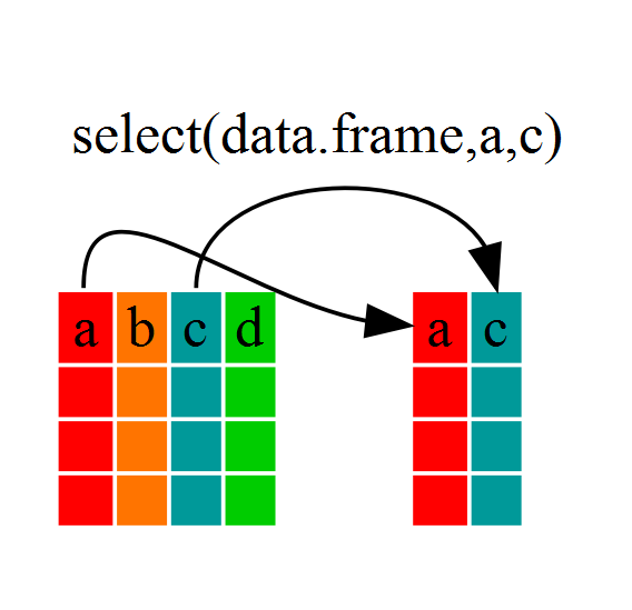
If we open up year_country_gdp, we will see that it only contains the year, country, and gdpPercap. This is equivalent to the base R subsetting function:
year_country_gdp_base <- gap[,c("year", "country", "gdpPercap")]
head(year_country_gdp)
#> # A tibble: 6 x 3
#>    year country     gdpPercap
#>   <int> <fct>           <dbl>
#> 1  1952 Afghanistan      779.
#> 2  1957 Afghanistan      821.
#> 3  1962 Afghanistan      853.
#> 4  1967 Afghanistan      836.
#> 5  1972 Afghanistan      740.
#> 6  1977 Afghanistan      786.
9.2.4 The Pipe

Above, we used what is called ‘normal’ grammar, but the strengths of dplyr lie in combining several functions using pipes.
In typical base R code, a simple operation might be written like:
A computer has no trouble understanding this, and your cupcakes will be made just fine, but a person has to read right to left to understand the order of operations – the opposite of how most Western languages are read – making it harder to understand what is being done!
To be more readable without pipes, we might break up this code into intermediate objects:
But this can clutter our environment with a lot of variables that are not very useful to us. Plus, these variables are often named very similar things (e.g., step, step1, step2…), which can lead to confusion and the creation of hard-to-track-down bugs.
Enter the Pipe…
The pipe makes it easier to read code by laying out operations from left to right – each line can be read like a line of a recipe for the perfect data frame!
Pipes take the input on the left side of the %>% symbol and pass it in as the first argument to the function on the right side.
With pipes, our cupcake example might be written like:
select & Pipe (%>%)
Let’s repeat what we did above with the Gapminder dataset using pipes:
First, we summon the gapminder data frame and pass it on to the next step using the pipe symbol %>%.
The second step is the select() function. In this case, we do not specify which data object we use in the call to select() since we have piped it in from the previous line.
Tips for Piping
Remember that you do not assign anything within the pipes — that is, you should not use
<-inside the piped operation. Only use<-at the beginning of your code if you want to save the output.Remember to add the pipe
%>%at the end of each line involved in the piped operation. A good rule of thumb: since RStudio will automatically indent lines of code that are part of a piped operation, if the line is not indented, it probably has not been added to the pipe. If you have an error in a piped operation, always check to make sure the pipe is connected as you expect.In RStudio, the hotkey for the pipe is
Ctrl + Shift + M.
9.2.5 Filter Rows with filter
Now let’s say we are only interested in African countries. We can combine select and filter to select only the observations where continent is Africa.
year_country_gdp_africa <- gap %>%
    filter(continent == "Africa") %>%
    select(year, country, gdpPercap)
As with last time, first we pass the gapminder dataframe to the filter() function, then we pass the filtered version of the Gapminder dataframe to the select() function.
To clarify, both the select and filter functions subset the data frame. The difference is that select extracts certain columns, while filter extracts certain rows.
NB: The order of operations is very important in this case. If we used select first, filter would not be able to find the variable continent, since we would have removed it in the previous step.
9.3 More dplyr functions
Where were we?
In the previous lesson, we used two very important verbs and an operator:
filter()for subsetting data with row logic.select()for subsetting data variable- or column-wise.- The pipe operator
%>%, which feeds the LHS as the first argument to the expression on the RHS.
We also discussed dplyr’s role inside the tidyverse:
dplyris a core package in the tidyverse meta-package.- Since we often make incidental usage of the others, we will load
dplyrand the others vialibrary(tidyverse).
9.3.1 Use mutate() to Add New Variables
Imagine we wanted to recover each country’s GDP. After all, the Gapminder data has a variable for population and GDP per capita. Let’s multiply them together.
mutate() is a function that defines and inserts new variables into a tibble. You can refer to existing variables by name.
gap %>%
  mutate(gdp = pop * gdpPercap) %>%
  head()
#> # A tibble: 6 x 7
#>   country     continent  year lifeExp      pop gdpPercap          gdp
#>   <fct>       <fct>     <int>   <dbl>    <int>     <dbl>        <dbl>
#> 1 Afghanistan Asia       1952    28.8  8425333      779.  6567086330.
#> 2 Afghanistan Asia       1957    30.3  9240934      821.  7585448670.
#> 3 Afghanistan Asia       1962    32.0 10267083      853.  8758855797.
#> 4 Afghanistan Asia       1967    34.0 11537966      836.  9648014150.
#> 5 Afghanistan Asia       1972    36.1 13079460      740.  9678553274.
#> 6 Afghanistan Asia       1977    38.4 14880372      786. 11697659231.
We can add multiple columns in one call:
gap %>%
  mutate(gdp = pop * gdpPercap,
         log_gdp = log(gdp)) %>%
  head()
#> # A tibble: 6 x 8
#>   country     continent  year lifeExp      pop gdpPercap          gdp log_gdp
#>   <fct>       <fct>     <int>   <dbl>    <int>     <dbl>        <dbl>   <dbl>
#> 1 Afghanistan Asia       1952    28.8  8425333      779.  6567086330.    22.6
#> 2 Afghanistan Asia       1957    30.3  9240934      821.  7585448670.    22.7
#> 3 Afghanistan Asia       1962    32.0 10267083      853.  8758855797.    22.9
#> 4 Afghanistan Asia       1967    34.0 11537966      836.  9648014150.    23.0
#> 5 Afghanistan Asia       1972    36.1 13079460      740.  9678553274.    23.0
#> 6 Afghanistan Asia       1977    38.4 14880372      786. 11697659231.    23.2
9.3.2 Use arrange() to Row-order Data in a Principled Way
arrange() reorders the rows in a data frame. Imagine you wanted this data ordered by year then country, as opposed to by country then year.
gap %>%
  arrange(year, country)
#> # A tibble: 1,704 x 6
#>   country     continent  year lifeExp      pop gdpPercap
#>   <fct>       <fct>     <int>   <dbl>    <int>     <dbl>
#> 1 Afghanistan Asia       1952    28.8  8425333      779.
#> 2 Albania     Europe     1952    55.2  1282697     1601.
#> 3 Algeria     Africa     1952    43.1  9279525     2449.
#> 4 Angola      Africa     1952    30.0  4232095     3521.
#> 5 Argentina   Americas   1952    62.5 17876956     5911.
#> 6 Australia   Oceania    1952    69.1  8691212    10040.
#> # … with 1,698 more rows
Or maybe you want just the data from 2007, sorted on life expectancy?
gap %>%
  filter(year == 2007) %>%
  arrange(lifeExp)
#> # A tibble: 142 x 6
#>   country      continent  year lifeExp      pop gdpPercap
#>   <fct>        <fct>     <int>   <dbl>    <int>     <dbl>
#> 1 Swaziland    Africa     2007    39.6  1133066     4513.
#> 2 Mozambique   Africa     2007    42.1 19951656      824.
#> 3 Zambia       Africa     2007    42.4 11746035     1271.
#> 4 Sierra Leone Africa     2007    42.6  6144562      863.
#> 5 Lesotho      Africa     2007    42.6  2012649     1569.
#> 6 Angola       Africa     2007    42.7 12420476     4797.
#> # … with 136 more rows
Oh, you would like to sort on life expectancy in descending order? Then use desc().
gap %>%
  filter(year == 2007) %>%
  arrange(desc(lifeExp))
#> # A tibble: 142 x 6
#>   country          continent  year lifeExp       pop gdpPercap
#>   <fct>            <fct>     <int>   <dbl>     <int>     <dbl>
#> 1 Japan            Asia       2007    82.6 127467972    31656.
#> 2 Hong Kong, China Asia       2007    82.2   6980412    39725.
#> 3 Iceland          Europe     2007    81.8    301931    36181.
#> 4 Switzerland      Europe     2007    81.7   7554661    37506.
#> 5 Australia        Oceania    2007    81.2  20434176    34435.
#> 6 Spain            Europe     2007    80.9  40448191    28821.
#> # … with 136 more rows
I advise that your analyses NEVER rely on rows or variables being in a specific order. But it is still true that human beings write the code, and the interactive development process can be much nicer if you reorder the rows of your data as you go along. Also, once you are preparing tables for human eyeballs, it is imperative that you step up and take control of row order.
9.3.3 Use rename() to Rename Variables
When I first cleaned this Gapminder excerpt, I was a camelCase person, but now I am all about snake_case. So I am vexed by the variable names I chose when I cleaned this data years ago. Let’s rename some variables!
gap %>%
  rename(life_exp = lifeExp,
         gdp_percap = gdpPercap)
#> # A tibble: 1,704 x 6
#>   country     continent  year life_exp      pop gdp_percap
#>   <fct>       <fct>     <int>    <dbl>    <int>      <dbl>
#> 1 Afghanistan Asia       1952     28.8  8425333       779.
#> 2 Afghanistan Asia       1957     30.3  9240934       821.
#> 3 Afghanistan Asia       1962     32.0 10267083       853.
#> 4 Afghanistan Asia       1967     34.0 11537966       836.
#> 5 Afghanistan Asia       1972     36.1 13079460       740.
#> 6 Afghanistan Asia       1977     38.4 14880372       786.
#> # … with 1,698 more rows
9.3.4 Use select() to Rename and Reposition Variables
You have seen the simple use of select(). There are two tricks you might enjoy:
select()can rename the variables you request to keep.select()can be used witheverything()to hoist a variable up to the front of the tibble.
gap %>%
  filter(country == "Burundi", year > 1996) %>%
  select(yr = year, lifeExp, gdpPercap) %>%
  select(gdpPercap, everything())
#> # A tibble: 3 x 3
#>   gdpPercap    yr lifeExp
#>       <dbl> <int>   <dbl>
#> 1      463.  1997    45.3
#> 2      446.  2002    47.4
#> 3      430.  2007    49.6
everything() is one of several helpers for variable selection. Read its help to see the rest.
9.3.5 Use count() to Count Variable Quantities
Finally, let’s say we want to examine if the number of countries covered in the Gapminder dataset varies between years. We can use count() to count the number of observations within a set of parameters we choose.
Below, we will specify that we want to count() the number of observations in each year of the dataset:
gap %>%
  dplyr::count(year)
#> # A tibble: 12 x 2
#>    year     n
#>   <int> <int>
#> 1  1952   142
#> 2  1957   142
#> 3  1962   142
#> 4  1967   142
#> 5  1972   142
#> 6  1977   142
#> # … with 6 more rows
We can confirm that each year in the dataset contains the same number of observations. We can use similar syntax to answer other questions: For example, how many countries in each year have a GDP that is greater than $10,000 per capita?
gap %>%
  filter(gdpPercap >= 10000) %>%
  dplyr::count(year)
#> # A tibble: 12 x 2
#>    year     n
#>   <int> <int>
#> 1  1952     7
#> 2  1957    12
#> 3  1962    19
#> 4  1967    22
#> 5  1972    32
#> 6  1977    41
#> # … with 6 more rowslibrary(tidyverse)
library(gapminder)
gap <- gapminder
head(gap)
#> # A tibble: 6 x 6
#> country continent year lifeExp pop gdpPercap
#> <fct> <fct> <int> <dbl> <int> <dbl>
#> 1 Afghanistan Asia 1952 28.8 8425333 779.
#> 2 Afghanistan Asia 1957 30.3 9240934 821.
#> 3 Afghanistan Asia 1962 32.0 10267083 853.
#> 4 Afghanistan Asia 1967 34.0 11537966 836.
#> 5 Afghanistan Asia 1972 36.1 13079460 740.
#> 6 Afghanistan Asia 1977 38.4 14880372 786.9.4 Calculating across Groups
A common task you will encounter when working with data is running calculations on different groups within the data. For instance, what if we wanted to calculate the mean GDP per capita for each continent?
In base R, you would have to run the mean() function for each subset of data.
mean(gap$gdpPercap[gap$continent == "Africa"])
#> [1] 2194
mean(gap$gdpPercap[gap$continent == "Americas"])
#> [1] 7136
mean(gap$gdpPercap[gap$continent == "Asia"])
#> [1] 7902
mean(gap$gdpPercap[gap$continent == "Europe"])
#> [1] 14469
mean(gap$gdpPercap[gap$continent == "Oceania"])
#> [1] 18622
That is a lot of repetition! To make matters worse, what if we wanted to add these values to our original data frame as a new column? We would have to write something like this:
gap$mean.continent.GDP <- NA
gap$mean.continent.GDP[gap$continent == "Africa"] <- mean(gap$gdpPercap[gap$continent == "Africa"])
gap$mean.continent.GDP[gap$continent == "Americas"] <- mean(gap$gdpPercap[gap$continent == "Americas"])
gap$mean.continent.GDP[gap$continent == "Asia"] <- mean(gap$gdpPercap[gap$continent == "Asia"])
gap$mean.continent.GDP[gap$continent == "Europe"] <- mean(gap$gdpPercap[gap$continent == "Europe"])
gap$mean.continent.GDP[gap$continent == "Oceania"] <- mean(gap$gdpPercap[gap$continent == "Oceania"])
You can see how this can get pretty tedious, especially if we want to calculate more complicated or refined statistics. We could use loops or apply functions, but these can be difficult, slow, and error-prone.
Split-apply-combine
The abstract problem we are encountering here is know as “split-apply-combine”:
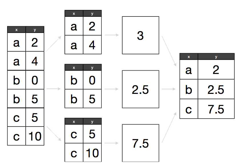
We want to split our data into groups (in this case, continents), apply some calculations on that group, then combine the results together afterwards.
Luckily, dplyr offers a much cleaner, straight-forward solution to this problem.
First, let’s remove the column we just made:
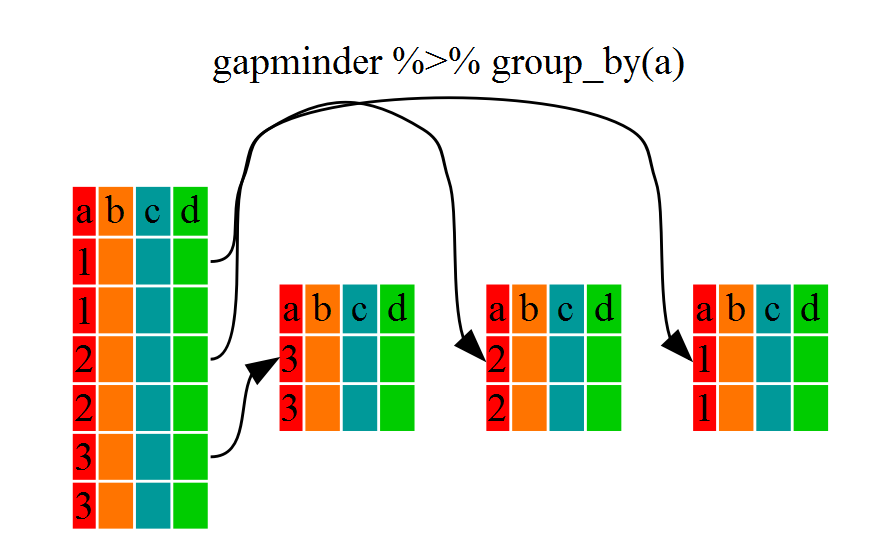
9.4.1 Use group_by to Create a Grouped Data
We have already seen how filter() can help us select observations that meet certain criteria (in the above: continent == "Africa"). More helpful, however, is the group_by() function, which will essentially use every unique criterium that we could have used in filter().
A grouped_df can be thought of as a list where each item in the list is a data.frame which contains only the rows that correspond to a particular value for continent (at least in the example above).
9.4.2 Summarize Across Groups with summarize
group_by() on its own is not particularly interesting. It is much more exciting used in conjunction with the summarize() function.
This will allow us to create new variable(s) by applying transformations to variables in each of our groups (continent-specific data frames).
In other words, using the group_by() function, we split our original data frame into multiple pieces, to which we then apply summary functions (e.g., mean() or sd()) within summarize().
The output is a new data frame reduced in size, with one row per group.
gap %>%
  group_by(continent) %>%
  summarize(mean_gdpPercap = mean(gdpPercap))
#> `summarise()` ungrouping output (override with `.groups` argument)
#> # A tibble: 5 x 2
#>   continent mean_gdpPercap
#>   <fct>              <dbl>
#> 1 Africa             2194.
#> 2 Americas           7136.
#> 3 Asia               7902.
#> 4 Europe            14469.
#> 5 Oceania           18622.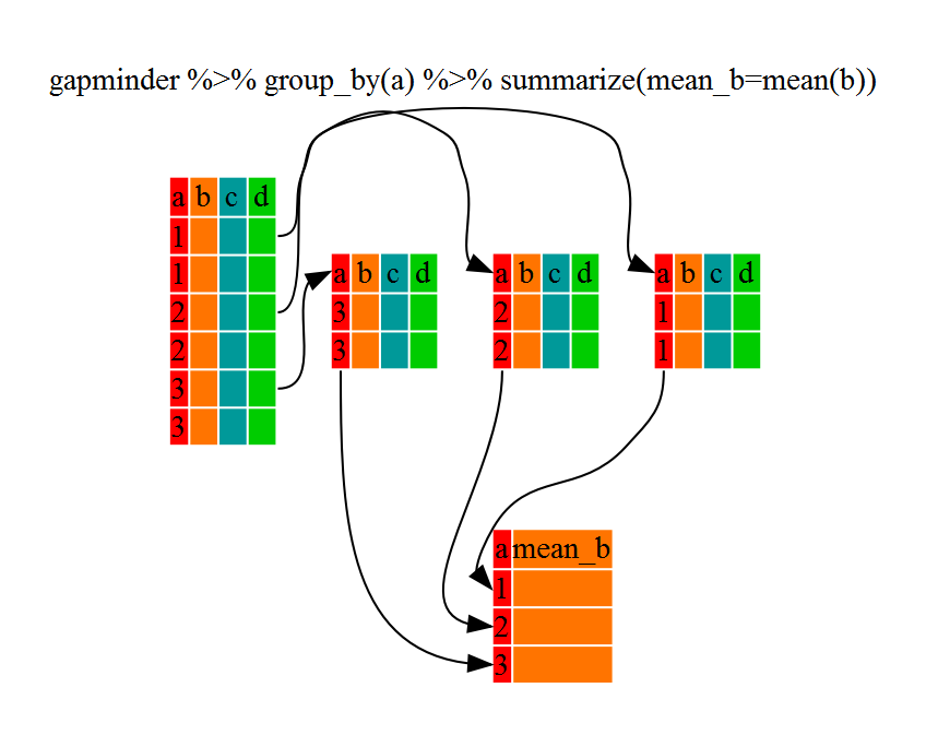
That allowed us to calculate the mean gdpPercap for each continent.
But it gets even better – the function group_by() allows us to group by multiple variables. Let’s group by year and continent:
gap %>%
  group_by(continent, year) %>%
  summarize(mean_gdpPercap = mean(gdpPercap)) %>%
  head()
#> `summarise()` regrouping output by 'continent' (override with `.groups` argument)
#> # A tibble: 6 x 3
#> # Groups:   continent [1]
#>   continent  year mean_gdpPercap
#>   <fct>     <int>          <dbl>
#> 1 Africa     1952          1253.
#> 2 Africa     1957          1385.
#> 3 Africa     1962          1598.
#> 4 Africa     1967          2050.
#> 5 Africa     1972          2340.
#> 6 Africa     1977          2586.
That is already quite powerful, but it gets even better! You are not limited to defining only one new variable in summarize().
gap %>%
  group_by(continent, year) %>%
  summarize(mean_gdpPercap = mean(gdpPercap),
            sd_gdpPercap = sd(gdpPercap),
            mean_pop = mean(pop),
            sd_pop = sd(pop))
#> `summarise()` regrouping output by 'continent' (override with `.groups` argument)
#> # A tibble: 60 x 6
#> # Groups:   continent [5]
#>   continent  year mean_gdpPercap sd_gdpPercap mean_pop    sd_pop
#>   <fct>     <int>          <dbl>        <dbl>    <dbl>     <dbl>
#> 1 Africa     1952          1253.         983. 4570010.  6317450.
#> 2 Africa     1957          1385.        1135. 5093033.  7076042.
#> 3 Africa     1962          1598.        1462. 5702247.  7957545.
#> 4 Africa     1967          2050.        2848. 6447875.  8985505.
#> 5 Africa     1972          2340.        3287. 7305376. 10130833.
#> 6 Africa     1977          2586.        4142. 8328097. 11585184.
#> # … with 54 more rows
9.4.3 Add New Variables with mutate
What if we wanted to add these values to our original data frame instead of creating a new object?
For this, we can use the mutate() function, which is similar to summarize() except that it creates new variables in the same data frame that you pass into it.
gap %>%
  group_by(continent, year) %>%
  mutate(mean_gdpPercap = mean(gdpPercap),
            sd_gdpPercap = sd(gdpPercap),
            mean_pop = mean(pop),
            sd_pop = sd(pop))
#> # A tibble: 1,704 x 10
#> # Groups:   continent, year [60]
#>   country continent  year lifeExp    pop gdpPercap mean_gdpPercap sd_gdpPercap
#>   <fct>   <fct>     <int>   <dbl>  <int>     <dbl>          <dbl>        <dbl>
#> 1 Afghan… Asia       1952    28.8 8.43e6      779.          5195.       18635.
#> 2 Afghan… Asia       1957    30.3 9.24e6      821.          5788.       19507.
#> 3 Afghan… Asia       1962    32.0 1.03e7      853.          5729.       16416.
#> 4 Afghan… Asia       1967    34.0 1.15e7      836.          5971.       14063.
#> 5 Afghan… Asia       1972    36.1 1.31e7      740.          8187.       19088.
#> 6 Afghan… Asia       1977    38.4 1.49e7      786.          7791.       11816.
#> # … with 1,698 more rows, and 2 more variables: mean_pop <dbl>, sd_pop <dbl>
We can also use mutate() to create new variables prior to (or even after) summarizing the information.
gap %>%
  mutate(gdp_billion = gdpPercap*pop/10^9) %>%
  group_by(continent, year) %>%
  summarize(mean_gdpPercap = mean(gdpPercap),
            sd_gdpPercap = sd(gdpPercap),
            mean_pop = mean(pop),
            sd_pop = sd(pop),
            mean_gdp_billion = mean(gdp_billion),
            sd_gdp_billion = sd(gdp_billion))
#> `summarise()` regrouping output by 'continent' (override with `.groups` argument)
#> # A tibble: 60 x 8
#> # Groups:   continent [5]
#>   continent  year mean_gdpPercap sd_gdpPercap mean_pop sd_pop mean_gdp_billion
#>   <fct>     <int>          <dbl>        <dbl>    <dbl>  <dbl>            <dbl>
#> 1 Africa     1952          1253.         983. 4570010. 6.32e6             5.99
#> 2 Africa     1957          1385.        1135. 5093033. 7.08e6             7.36
#> 3 Africa     1962          1598.        1462. 5702247. 7.96e6             8.78
#> 4 Africa     1967          2050.        2848. 6447875. 8.99e6            11.4
#> 5 Africa     1972          2340.        3287. 7305376. 1.01e7            15.1
#> 6 Africa     1977          2586.        4142. 8328097. 1.16e7            18.7
#> # … with 54 more rows, and 1 more variable: sd_gdp_billion <dbl>
mutate vs. summarize
It can be confusing to decide whether to use mutate or summarize. The key distinction is whether you want the output to have one row for each group or one row for each row in the original data frame:
mutate: Creates new columns with as many rows as the original data frame.summarize: Creates a data frame with as many rows as groups.
Note that if you use an aggregation function such as mean() within mutate() without using group_by(), you will simply do the summary over all the rows of the input data frame.
And if you use an aggregation function such as mean() within summarize() without using group_by(), you will simply create an output data frame with one row (i.e., the whole input data frame is a single group).
9.5 Challenges
Challenge 1.
Use dplyr to create a data frame containing the median lifeExp for each continent.
Challenge 2.
Use dplyr to add a column to the Gapminder dataset that contains the total population of the continent of each observation in a given year. For example, if the first observation is Afghanistan in 1952, the new column would contain the population of Asia in 1952.
Challenge 3.
Use dplyr to: (a) add a column called gdpPercap_diff that contains the difference between the observation’s gdpPercap and the mean gdpPercap of the continent in that year, and (b) arrange the data frame by the column you just created in descending order (so that the relatively richest country-years are listed first).
Acknowledgments
Some of the materials in this module were adapted from: