Chapter 13 Statistical Inferences
13.1 Statistical Distributions
Since R was developed by statisticians, it handles distributions and simulation seamlessly.
All commonly-used distributions have functions in R. Each distribution has a family of functions:
d- Probability density/mass function, e.g.,dnorm()r- Generate a random value, e.g.,rnorm()p- Cumulative distribution function, e.g.,pnorm()q- Quantile function (inverse CDF), e.g.,qnorm()
Let’s see some of these functions in action with the normal distribution (mean 0, standard deviation 1):
dnorm(1.96) # Probability density of 1.96 from the normal distribution
#> [1] 0.0584
rnorm(1:10) # Get 10 random values from the normal distribution
#>  [1] -1.40004  0.25532 -2.43726 -0.00557  0.62155  1.14841 -1.82182 -0.24733
#>  [9] -0.24420 -0.28271
pnorm(1.96) # Cumulative distribution function
#> [1] 0.975
qnorm(.975) # Inverse cumulative distribution function
#> [1] 1.96
We can also use these functions on other distributions:
rnorm()# Normal distributionrunif()# Uniform distributionrbinom()# Binomial distributionrpois()# Poisson distributionrbeta()# Beta distributionrgamma()# Gamma distributionrt()# Student t distributionrchisq(). # Chi-squared distribution
rbinom(0:10, size = 10, prob = 0.3)
#>  [1] 2 4 4 2 6 4 1 3 4 4 1
dt(5, df = 1)
#> [1] 0.0122

x <- seq(-5, 5, length = 100)
plot(x, dnorm(x), type = 'l')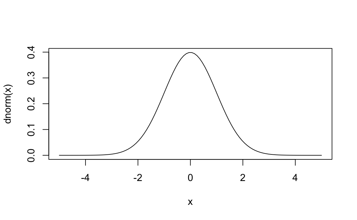
13.1.1 Sampling and Simulation
We can draw a sample with or without replacement with sample.
sample(1:nrow(gap), 20, replace = FALSE)
#>  [1]  447 1284  752  674 1699 1241  726 1579 1568 1094  265  150 1023 1290 1440
#> [16]  117  930 1553  180 1208
dplyr has a helpful select_n function that samples rows of a dataframe.
Here’s an example of some code that would be part of a bootstrap:
13.1.2 Random Seeds
A few key facts about generating random numbers:
- Random numbers on a computer are pseudo-random; they are generated deterministically from a very, very, very long sequence that repeats.
- The seed determines where you are in that sequence.
To replicate any work involving random numbers, make sure to set the seed first. The seed can be arbitrary – pick your favorite number.
13.1.3 Challenges
Challenge 1.
Generate 100 random Poisson values with a population mean of 5. How close is the mean of those 100 values to the value of 5?
Challenge 2.
What is the 95th percentile of a chi-square distribution with 1 degree of freedom?
Challenge 3.
What is the probability of getting a value greater than 5 if you draw from a standard normal distribution? What about a t distribution with 1 degree of freedom?
13.2 Inferences and Regressions
Once we have imported our data, summarized it, carried out group-wise operations, and perhaps reshaped it, we may also want to attempt causal inference.
This often requires doing the following:
- Carrying out hypothesis tests
- Estimating regression models
13.2.1 Statistical Tests
Let’s say we are interested in whether the life expectancy in 1967 is different than in 1977.
NB: pull() is a dplyr method to select a single variable as store it as a 1d vector.
# Pull out life expectancy by different years
lifeExp_1967 <- gap %>%
  filter(year==1967) %>%
  pull(lifeExp)

lifeExp_1977 <- gap %>%
  filter(year==1977) %>%
  pull(lifeExp)
One can test for differences in distributions in either:
- Their means using t-tests:
# t test of means
t.test(x = lifeExp_1967, y = lifeExp_1977)
#>
#>  Welch Two Sample t-test
#>
#> data:  lifeExp_1967 and lifeExp_1977
#> t = -3, df = 281, p-value = 0.005
#> alternative hypothesis: true difference in means is not equal to 0
#> 95 percent confidence interval:
#>  -6.57 -1.21
#> sample estimates:
#> mean of x mean of y
#> 55.7 59.6- Their entire distributions using ks-tests:
13.2.2 Regressions and Linear Models
Running regressions in R is generally straightforward. There are two basic, catch-all regression functions in R:
lmfits a standard linear regression with OLS (equivalent toglmwithfamily = gaussian(link = "identity")).glmfits a generalized linear model with your choice of family/link function.
There are a bunch of families and links to use (?family for a full list), but some essentials are:
binomial(link = "logit"),gaussian(link = "identity")poisson(link = "log").
Formulas
We specify the statistical relationships to fit using a formula. The variable on the left-hand side of a tilde (~) is called the “dependent variable”, while the variables on the right-hand side are called the “independent variables” and are joined by plus signs + (for a basic linear combination).
Example: Suppose we want to regress life expectancy on GDP per capita and population, as well as continent and year.
The lm call looks something like this:
The glm call would look something like this:
mod <- glm(formula = lifeExp ~ log(gdpPercap) + log(pop) + continent + year,
           data = gap,
           family = gaussian(link = "identity"))
In addition to the + symbol, there are also other operators to control your formulas:
- for removing terms;
: for interaction;
* for crossing;
. for all other variables in the dataframe that haven’t yet been included in the model.
Let’s see some of these in action:
# `.` includes all  variables but `-` removes specific terms:
mod.1 <- lm(lifeExp ~ . - country,
            data = gap)
summary(mod.1)
#>
#> Call:
#> lm(formula = lifeExp ~ . - country, data = gap)
#>
#> Residuals:
#>     Min      1Q  Median      3Q     Max
#> -28.405  -4.055   0.232   4.507  20.022
#>
#> Coefficients:
#>                    Estimate Std. Error t value Pr(>|t|)
#> (Intercept)       -5.18e+02   1.99e+01   -26.1   <2e-16 ***
#> continentAmericas  1.43e+01   4.95e-01    28.9   <2e-16 ***
#> continentAsia      9.38e+00   4.72e-01    19.9   <2e-16 ***
#> continentEurope    1.94e+01   5.18e-01    37.4   <2e-16 ***
#> continentOceania   2.06e+01   1.47e+00    14.0   <2e-16 ***
#> year               2.86e-01   1.01e-02    28.5   <2e-16 ***
#> pop                1.79e-09   1.63e-09     1.1     0.27
#> gdpPercap          2.98e-04   2.00e-05    14.9   <2e-16 ***
#> ---
#> Signif. codes:  0 '***' 0.001 '**' 0.01 '*' 0.05 '.' 0.1 ' ' 1
#>
#> Residual standard error: 6.88 on 1696 degrees of freedom
#> Multiple R-squared:  0.717,  Adjusted R-squared:  0.716
#> F-statistic:  614 on 7 and 1696 DF,  p-value: <2e-16

# `x1:x2` interacts all terms in `x1` with all terms in `x2`:
mod.2 <- lm(lifeExp ~ log(gdpPercap) + log(pop) + continent:factor(year),
            data = gap)
summary(mod.2)
#>
#> Call:
#> lm(formula = lifeExp ~ log(gdpPercap) + log(pop) + continent:factor(year),
#>     data = gap)
#>
#> Residuals:
#>     Min      1Q  Median      3Q     Max
#> -26.568  -2.553   0.004   2.915  15.567
#>
#> Coefficients: (1 not defined because of singularities)
#>                                    Estimate Std. Error t value Pr(>|t|)
#> (Intercept)                         27.1838     4.6849    5.80  7.8e-09 ***
#> log(gdpPercap)                       5.0795     0.1605   31.65  < 2e-16 ***
#> log(pop)                             0.0789     0.0943    0.84  0.40251
#> continentAfrica:factor(year)1952   -24.1425     4.1125   -5.87  5.2e-09 ***
#> continentAmericas:factor(year)1952 -16.4465     4.1663   -3.95  8.2e-05 ***
#> continentAsia:factor(year)1952     -19.3347     4.1408   -4.67  3.3e-06 ***
#> continentEurope:factor(year)1952    -7.0918     4.1352   -1.71  0.08654 .
#> continentOceania:factor(year)1952   -6.0635     5.6511   -1.07  0.28344
#> continentAfrica:factor(year)1957   -22.4964     4.1098   -5.47  5.1e-08 ***
#> continentAmericas:factor(year)1957 -14.3673     4.1643   -3.45  0.00057 ***
#> continentAsia:factor(year)1957     -17.1743     4.1375   -4.15  3.5e-05 ***
#> continentEurope:factor(year)1957    -5.9094     4.1327   -1.43  0.15293
#> continentOceania:factor(year)1957   -5.6300     5.6503   -1.00  0.31921
#> continentAfrica:factor(year)1962   -21.0139     4.1069   -5.12  3.5e-07 ***
#> continentAmericas:factor(year)1962 -12.3135     4.1630   -2.96  0.00314 **
#> continentAsia:factor(year)1962     -15.5626     4.1351   -3.76  0.00017 ***
#> continentEurope:factor(year)1962    -5.0542     4.1308   -1.22  0.22130
#> continentOceania:factor(year)1962   -5.3122     5.6498   -0.94  0.34723
#> continentAfrica:factor(year)1967   -19.7034     4.1035   -4.80  1.7e-06 ***
#> continentAmericas:factor(year)1967 -10.9324     4.1613   -2.63  0.00869 **
#> continentAsia:factor(year)1967     -13.1569     4.1327   -3.18  0.00148 **
#> continentEurope:factor(year)1967    -4.9134     4.1291   -1.19  0.23423
#> continentOceania:factor(year)1967   -5.7712     5.6492   -1.02  0.30712
#> continentAfrica:factor(year)1972   -18.1469     4.1007   -4.43  1.0e-05 ***
#> continentAmericas:factor(year)1972  -9.6537     4.1595   -2.32  0.02042 *
#> continentAsia:factor(year)1972     -11.6014     4.1293   -2.81  0.00502 **
#> continentEurope:factor(year)1972    -4.9763     4.1275   -1.21  0.22813
#> continentOceania:factor(year)1972   -5.8094     5.6487   -1.03  0.30389
#> continentAfrica:factor(year)1977   -16.1848     4.0996   -3.95  8.2e-05 ***
#> continentAmericas:factor(year)1977  -8.3382     4.1580   -2.01  0.04509 *
#> continentAsia:factor(year)1977     -10.1220     4.1270   -2.45  0.01428 *
#> continentEurope:factor(year)1977    -4.5523     4.1267   -1.10  0.27013
#> continentOceania:factor(year)1977   -5.1232     5.6485   -0.91  0.36454
#> continentAfrica:factor(year)1982   -14.1933     4.0990   -3.46  0.00055 ***
#> continentAmericas:factor(year)1982  -6.5921     4.1577   -1.59  0.11304
#> continentAsia:factor(year)1982      -7.6001     4.1257   -1.84  0.06564 .
#> continentEurope:factor(year)1982    -4.1185     4.1262   -1.00  0.31837
#> continentOceania:factor(year)1982   -4.0553     5.6483   -0.72  0.47288
#> continentAfrica:factor(year)1987   -12.1850     4.0995   -2.97  0.00300 **
#> continentAmericas:factor(year)1987  -4.7157     4.1577   -1.13  0.25687
#> continentAsia:factor(year)1987      -5.6914     4.1249   -1.38  0.16785
#> continentEurope:factor(year)1987    -3.7298     4.1258   -0.90  0.36613
#> continentOceania:factor(year)1987   -3.5164     5.6480   -0.62  0.53364
#> continentAfrica:factor(year)1992   -11.8028     4.0994   -2.88  0.00404 **
#> continentAmericas:factor(year)1992  -3.2855     4.1575   -0.79  0.42949
#> continentAsia:factor(year)1992      -4.3823     4.1241   -1.06  0.28811
#> continentEurope:factor(year)1992    -2.5151     4.1262   -0.61  0.54225
#> continentOceania:factor(year)1992   -1.9804     5.6480   -0.35  0.72590
#> continentAfrica:factor(year)1997   -11.9577     4.0986   -2.92  0.00358 **
#> continentAmericas:factor(year)1997  -2.1611     4.1566   -0.52  0.60319
#> continentAsia:factor(year)1997      -3.5016     4.1228   -0.85  0.39583
#> continentEurope:factor(year)1997    -2.0843     4.1256   -0.51  0.61348
#> continentOceania:factor(year)1997   -1.4478     5.6478   -0.26  0.79771
#> continentAfrica:factor(year)2002   -12.5237     4.0972   -3.06  0.00227 **
#> continentAmericas:factor(year)2002  -0.9898     4.1564   -0.24  0.81180
#> continentAsia:factor(year)2002      -2.6798     4.1221   -0.65  0.51571
#> continentEurope:factor(year)2002    -1.5734     4.1252   -0.38  0.70294
#> continentOceania:factor(year)2002   -0.4735     5.6477   -0.08  0.93320
#> continentAfrica:factor(year)2007   -11.6568     4.0948   -2.85  0.00447 **
#> continentAmericas:factor(year)2007  -0.6931     4.1550   -0.17  0.86754
#> continentAsia:factor(year)2007      -2.2008     4.1202   -0.53  0.59332
#> continentEurope:factor(year)2007    -1.5284     4.1247   -0.37  0.71102
#> continentOceania:factor(year)2007        NA         NA      NA       NA
#> ---
#> Signif. codes:  0 '***' 0.001 '**' 0.01 '*' 0.05 '.' 0.1 ' ' 1
#>
#> Residual standard error: 5.65 on 1642 degrees of freedom
#> Multiple R-squared:  0.816,  Adjusted R-squared:  0.809
#> F-statistic:  119 on 61 and 1642 DF,  p-value: <2e-16

# `x1*x2` produces the cross of `x1` and `x2`, or `x1 + x2 + x1:x2`:
mod.3 <- lm(lifeExp ~ log(gdpPercap) + log(pop) + continent*factor(year),
            data = gap)
summary(mod.3)
#>
#> Call:
#> lm(formula = lifeExp ~ log(gdpPercap) + log(pop) + continent *
#>     factor(year), data = gap)
#>
#> Residuals:
#>     Min      1Q  Median      3Q     Max
#> -26.568  -2.553   0.004   2.915  15.567
#>
#> Coefficients:
#>                                    Estimate Std. Error t value Pr(>|t|)
#> (Intercept)                          3.0413     2.0741    1.47  0.14275
#> log(gdpPercap)                       5.0795     0.1605   31.65  < 2e-16 ***
#> log(pop)                             0.0789     0.0943    0.84  0.40251
#> continentAmericas                    7.6960     1.3932    5.52  3.9e-08 ***
#> continentAsia                        4.8078     1.2657    3.80  0.00015 ***
#> continentEurope                     17.0508     1.3295   12.83  < 2e-16 ***
#> continentOceania                    18.0790     4.0890    4.42  1.0e-05 ***
#> factor(year)1957                     1.6461     1.1078    1.49  0.13747
#> factor(year)1962                     3.1286     1.1084    2.82  0.00482 **
#> factor(year)1967                     4.4392     1.1097    4.00  6.6e-05 ***
#> factor(year)1972                     5.9956     1.1113    5.39  7.9e-08 ***
#> factor(year)1977                     7.9578     1.1124    7.15  1.3e-12 ***
#> factor(year)1982                     9.9492     1.1134    8.94  < 2e-16 ***
#> factor(year)1987                    11.9575     1.1138   10.74  < 2e-16 ***
#> factor(year)1992                    12.3398     1.1146   11.07  < 2e-16 ***
#> factor(year)1997                    12.1848     1.1161   10.92  < 2e-16 ***
#> factor(year)2002                    11.6188     1.1181   10.39  < 2e-16 ***
#> factor(year)2007                    12.4857     1.1212   11.14  < 2e-16 ***
#> continentAmericas:factor(year)1957   0.4330     1.9438    0.22  0.82375
#> continentAsia:factor(year)1957       0.5142     1.7776    0.29  0.77241
#> continentEurope:factor(year)1957    -0.4638     1.8313   -0.25  0.80010
#> continentOceania:factor(year)1957   -1.2126     5.7552   -0.21  0.83315
#> continentAmericas:factor(year)1962   1.0043     1.9438    0.52  0.60546
#> continentAsia:factor(year)1962       0.6435     1.7777    0.36  0.71741
#> continentEurope:factor(year)1962    -1.0911     1.8315   -0.60  0.55142
#> continentOceania:factor(year)1962   -2.3774     5.7552   -0.41  0.67960
#> continentAmericas:factor(year)1967   1.0750     1.9438    0.55  0.58033
#> continentAsia:factor(year)1967       1.7387     1.7777    0.98  0.32819
#> continentEurope:factor(year)1967    -2.2608     1.8317   -1.23  0.21728
#> continentOceania:factor(year)1967   -4.1468     5.7552   -0.72  0.47130
#> continentAmericas:factor(year)1972   0.7972     1.9438    0.41  0.68176
#> continentAsia:factor(year)1972       1.7377     1.7779    0.98  0.32851
#> continentEurope:factor(year)1972    -3.8801     1.8322   -2.12  0.03435 *
#> continentOceania:factor(year)1972   -5.7415     5.7552   -1.00  0.31862
#> continentAmericas:factor(year)1977   0.1505     1.9439    0.08  0.93828
#> continentAsia:factor(year)1977       1.2549     1.7784    0.71  0.48050
#> continentEurope:factor(year)1977    -5.4183     1.8329   -2.96  0.00316 **
#> continentOceania:factor(year)1977   -7.0175     5.7553   -1.22  0.22290
#> continentAmericas:factor(year)1982  -0.0948     1.9439   -0.05  0.96110
#> continentAsia:factor(year)1982       1.7854     1.7788    1.00  0.31567
#> continentEurope:factor(year)1982    -6.9759     1.8336   -3.80  0.00015 ***
#> continentOceania:factor(year)1982   -7.9409     5.7553   -1.38  0.16785
#> continentAmericas:factor(year)1987  -0.2267     1.9440   -0.12  0.90720
#> continentAsia:factor(year)1987       1.6858     1.7796    0.95  0.34363
#> continentEurope:factor(year)1987    -8.5955     1.8350   -4.68  3.0e-06 ***
#> continentOceania:factor(year)1987   -9.4104     5.7554   -1.64  0.10223
#> continentAmericas:factor(year)1992   0.8213     1.9441    0.42  0.67276
#> continentAsia:factor(year)1992       2.6127     1.7803    1.47  0.14243
#> continentEurope:factor(year)1992    -7.7631     1.8346   -4.23  2.5e-05 ***
#> continentOceania:factor(year)1992   -8.2567     5.7555   -1.43  0.15160
#> continentAmericas:factor(year)1997   2.1006     1.9443    1.08  0.28012
#> continentAsia:factor(year)1997       3.6483     1.7812    2.05  0.04070 *
#> continentEurope:factor(year)1997    -7.1773     1.8358   -3.91  9.6e-05 ***
#> continentOceania:factor(year)1997   -7.5691     5.7557   -1.32  0.18867
#> continentAmericas:factor(year)2002   3.8379     1.9442    1.97  0.04854 *
#> continentAsia:factor(year)2002       5.0361     1.7814    2.83  0.00476 **
#> continentEurope:factor(year)2002    -6.1005     1.8369   -3.32  0.00092 ***
#> continentOceania:factor(year)2002   -6.0287     5.7558   -1.05  0.29506
#> continentAmericas:factor(year)2007   3.2677     1.9444    1.68  0.09303 .
#> continentAsia:factor(year)2007       4.6483     1.7823    2.61  0.00919 **
#> continentEurope:factor(year)2007    -6.9223     1.8378   -3.77  0.00017 ***
#> continentOceania:factor(year)2007   -6.4222     5.7558   -1.12  0.26468
#> ---
#> Signif. codes:  0 '***' 0.001 '**' 0.01 '*' 0.05 '.' 0.1 ' ' 1
#>
#> Residual standard error: 5.65 on 1642 degrees of freedom
#> Multiple R-squared:  0.816,  Adjusted R-squared:  0.809
#> F-statistic:  119 on 61 and 1642 DF,  p-value: <2e-16
Categorical variables (Factors)
Note that we wrapped the year variable into a factor() function. By default, R breaks up our variables into their different factor levels (as it will do whenever your regressors have factor levels).
If your data are not factorized, you can tell lm/glm to factorize a variable (i.e., create dummy variables on the fly) by writing factor().
Missing values
Missing values obviously cannot convey any information about the relationship between the variables. Most modeling functions will drop any rows that contain missing values.
13.2.3 Regression Output
When we store this regression in an object, we get access to several items of interest.
First, R has a helpful summary method for regression objects:
summary(mod)
#>
#> Call:
#> lm(formula = lifeExp ~ log(gdpPercap) + log(pop) + continent +
#>     year, data = gap)
#>
#> Residuals:
#>     Min      1Q  Median      3Q     Max
#> -25.057  -3.286   0.329   3.706  15.065
#>
#> Coefficients:
#>                    Estimate Std. Error t value Pr(>|t|)
#> (Intercept)       -4.61e+02   1.70e+01  -27.15   <2e-16 ***
#> log(gdpPercap)     5.08e+00   1.63e-01   31.19   <2e-16 ***
#> log(pop)           1.53e-01   9.67e-02    1.58     0.11
#> continentAmericas  8.75e+00   4.77e-01   18.35   <2e-16 ***
#> continentAsia      6.83e+00   4.23e-01   16.13   <2e-16 ***
#> continentEurope    1.23e+01   5.29e-01   23.20   <2e-16 ***
#> continentOceania   1.25e+01   1.28e+00    9.79   <2e-16 ***
#> year               2.38e-01   8.93e-03   26.61   <2e-16 ***
#> ---
#> Signif. codes:  0 '***' 0.001 '**' 0.01 '*' 0.05 '.' 0.1 ' ' 1
#>
#> Residual standard error: 5.81 on 1696 degrees of freedom
#> Multiple R-squared:  0.798,  Adjusted R-squared:  0.798
#> F-statistic:  960 on 7 and 1696 DF,  p-value: <2e-16
We can also extract specific information from the model object itself:
- All components contained in the regression output:
names(mod)
#>  [1] "coefficients"  "residuals"     "effects"       "rank"
#>  [5] "fitted.values" "assign"        "qr"            "df.residual"
#>  [9] "contrasts"     "xlevels"       "call"          "terms"
#> [13] "model"- Regression coefficients:
mod$coefficients
#>       (Intercept)    log(gdpPercap)          log(pop) continentAmericas
#>          -460.813             5.076             0.153             8.745
#>     continentAsia   continentEurope  continentOceania              year
#> 6.825 12.281 12.540 0.238- Regression degrees of freedom:
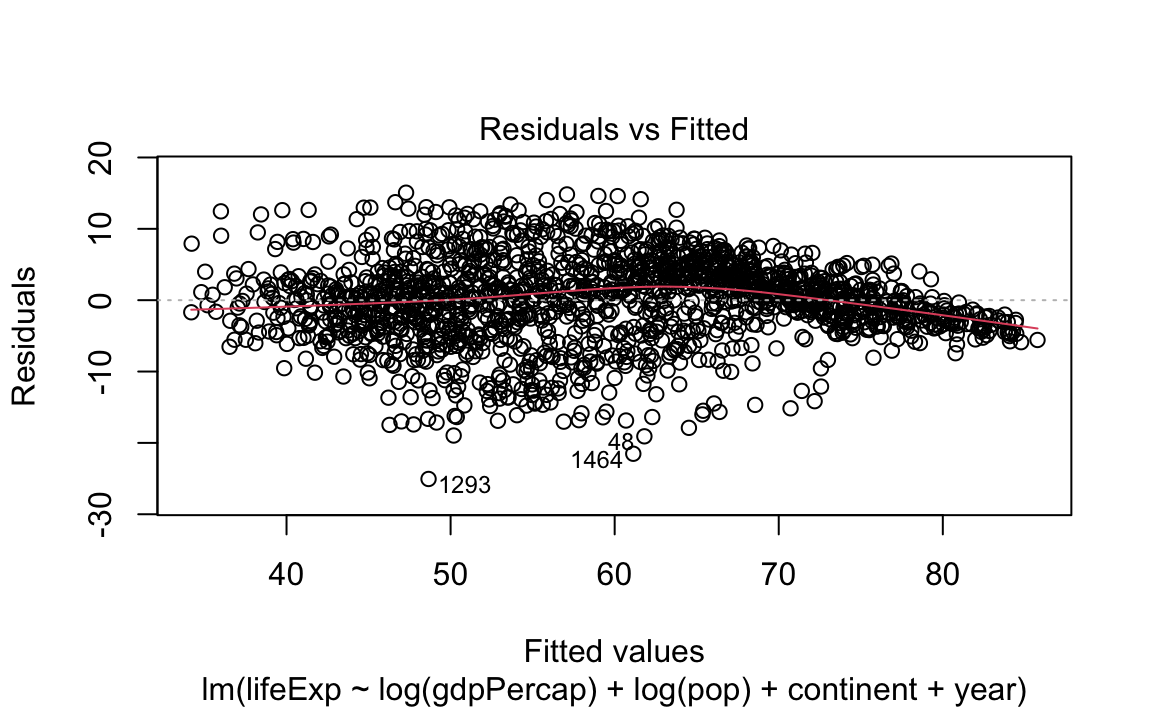
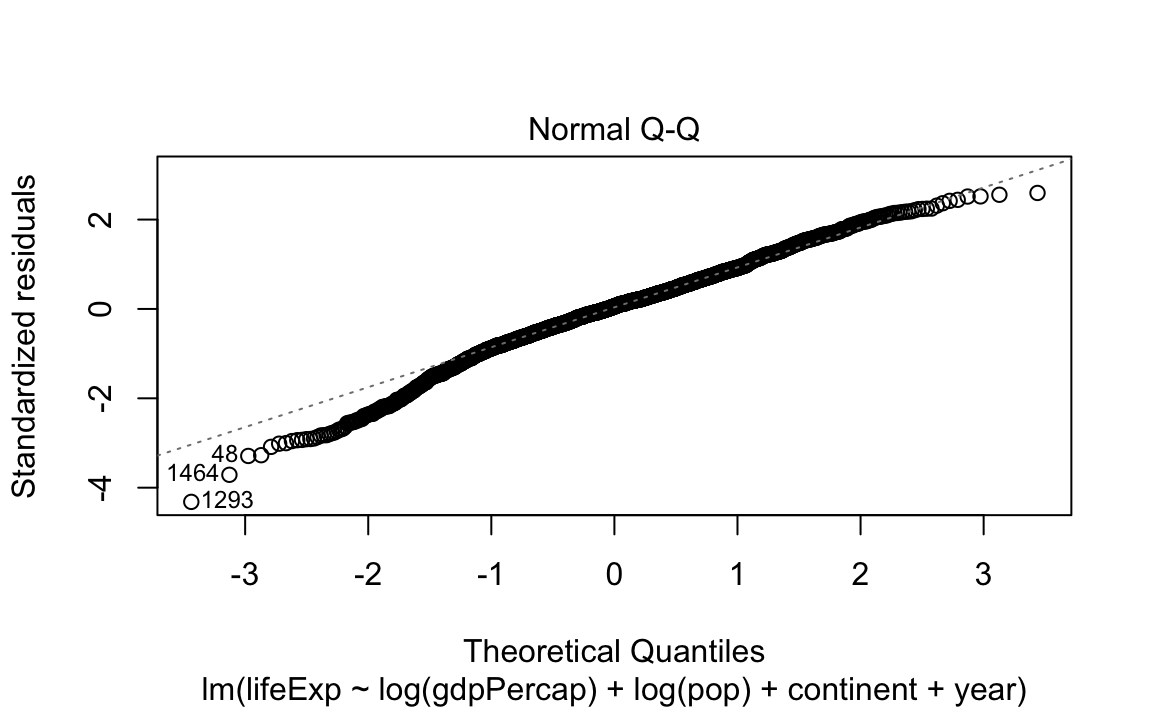
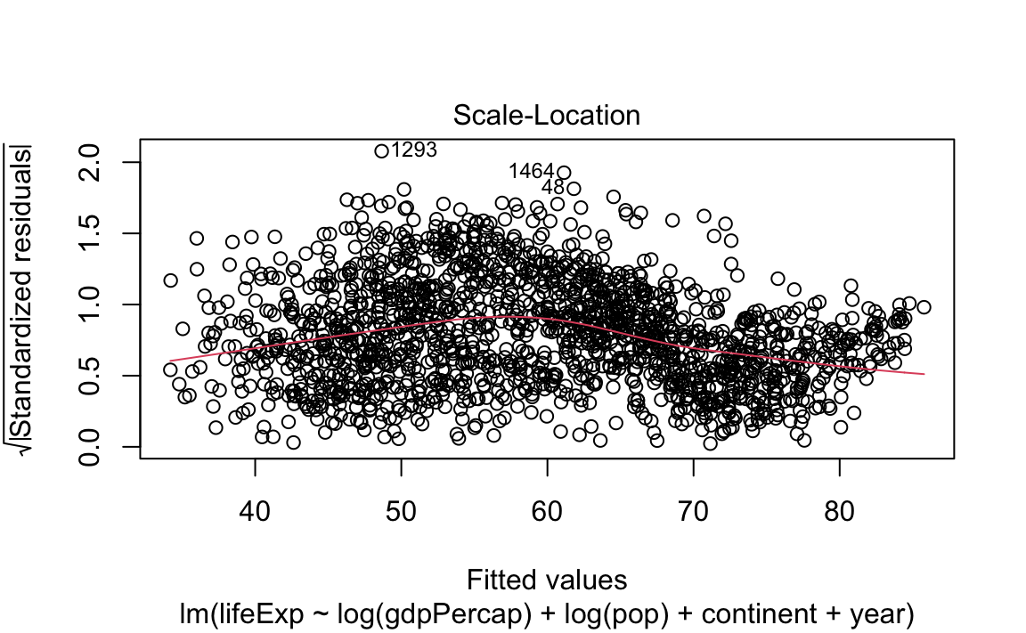
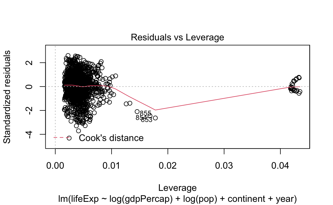
- Standard (diagnostic) plots for a regression:
13.2.4 Tidying model data with broom
The broom package, by David Robinson, turn models into tidy data.
broom::tidy(model) returns a row for each coefficient in the model. Each column gives information about the estimate or its variability.
mod_tidy <- tidy(mod)
mod_tidy
#> # A tibble: 8 x 5
#>   term              estimate std.error statistic   p.value
#>   <chr>                <dbl>     <dbl>     <dbl>     <dbl>
#> 1 (Intercept)       -461.      17.0       -27.2  3.96e-135
#> 2 log(gdpPercap)       5.08     0.163      31.2  3.37e-169
#> 3 log(pop)             0.153    0.0967      1.58 1.14e-  1
#> 4 continentAmericas    8.75     0.477      18.3  9.61e- 69
#> 5 continentAsia        6.83     0.423      16.1  1.49e- 54
#> 6 continentEurope     12.3      0.529      23.2  1.12e-103
#> # … with 2 more rows
This is a powerful technique for working with large numbers of models because once you have tidy data, you can apply all of the techniques that you’ve learned about earlier in the book.
13.2.5 Formatting Regression Tables
Most papers report the results of regression analysis in some kind of table. Typically, this table includes the values of coefficients, standard errors, and significance levels from one or more models.
The stargazer package provides excellent tools to make and format regression tables automatically. It can also output summary statistics from a dataframe.
library(stargazer)
stargazer(gap, type = "text")
#>
#> ===================================================
#> Statistic N Mean St. Dev. Min Pctl(25) Pctl(75) Max
#> ===================================================
Let’s say we want to report the results from three different models:
mod.1 <- lm(lifeExp ~ log(gdpPercap) + log(pop), data = gap)
mod.2 <- lm(lifeExp ~ log(gdpPercap) + log(pop) + continent, data = gap)
mod.3 <- lm(lifeExp ~ log(gdpPercap) + log(pop) + continent + year, data = gap)
stargazer can produce well-formatted tables that hold regression analysis results from all these models side-by-side.
stargazer(mod.1, mod.2, mod.3, title = "Regression Results", type = "text")
#>
#> Regression Results
#> ===================================================================================================
#>                                                   Dependent variable:
#>                     -------------------------------------------------------------------------------
#>                                                         lifeExp
#>                                 (1)                        (2)                       (3)
#> ---------------------------------------------------------------------------------------------------
#> log(gdpPercap)               8.340***                   6.590***                  5.080***
#>                               (0.143)                    (0.182)                   (0.163)
#>
#> log(pop)                     1.280***                   0.866***                    0.153
#>                               (0.111)                    (0.111)                   (0.097)
#>
#> continentAmericas                                       6.170***                  8.740***
#>                                                          (0.555)                   (0.477)
#>
#> continentAsia                                           4.670***                  6.830***
#>                                                          (0.494)                   (0.423)
#>
#> continentEurope                                         8.560***                  12.300***
#>                                                          (0.608)                   (0.529)
#>
#> continentOceania                                        8.350***                  12.500***
#>                                                          (1.510)                   (1.280)
#>
#> year                                                                              0.238***
#>                                                                                    (0.009)
#>
#> Constant                    -28.800***                 -12.000***                -461.000***
#>                               (2.080)                    (2.270)                  (17.000)
#>
#> ---------------------------------------------------------------------------------------------------
#> Observations                   1,704                      1,704                     1,704
#> R2                             0.677                      0.714                     0.798
#> Adjusted R2                    0.677                      0.713                     0.798
#> Residual Std. Error      7.340 (df = 1701)          6.920 (df = 1697)         5.810 (df = 1696)
#> F Statistic         1,786.000*** (df = 2; 1701) 707.000*** (df = 6; 1697) 960.000*** (df = 7; 1696)
#> ===================================================================================================
#> Note:                                                                   *p<0.1; **p<0.05; ***p<0.01
Customization
stargazer is incredibly customizable. Let’s say we wanted to
- Re-name our explanatory variables;
- Remove information on the “Constant”;
- Only keep the number of observations from the summary statistics; and
- Style the table to look like those in the American Journal of Political Science.
stargazer(mod.1, mod.2, mod.3, title = "Regression Results", type = "text",
          covariate.labels  = c("GDP per capita, logged", "Population, logged", "Americas", "Asia", "Europe", "Oceania", "Year", "Constant"),
          omit = "Constant",
          keep.stat="n", style = "ajps")
#>
#> Regression Results
#> --------------------------------------------------
#>                                  lifeExp
#>                        Model 1  Model 2   Model 3
#> --------------------------------------------------
#> GDP per capita, logged 8.340*** 6.590*** 5.080***
#>                        (0.143)  (0.182)   (0.163)
#> Population, logged     1.280*** 0.866***   0.153
#>                        (0.111)  (0.111)   (0.097)
#> Americas                        6.170*** 8.740***
#>                                 (0.555)   (0.477)
#> Asia                            4.670*** 6.830***
#>                                 (0.494)   (0.423)
#> Europe                          8.560*** 12.300***
#>                                 (0.608)   (0.529)
#> Oceania                         8.350*** 12.500***
#>                                 (1.510)   (1.280)
#> Year                                     0.238***
#>                                           (0.009)
#> N                        1704     1704     1704
#> --------------------------------------------------
#> ***p < .01; **p < .05; *p < .1
Check out ?stargazer to see more options.
Output Types
Once we like the look of our table, we can output/export it in a number of ways. The type argument specifies what output the command should produce. Possible values are:
"latex"for LaTeX code."html"for HTML code."text"for ASCII text output (what we used above).
Let’s say we are using LaTeX to typeset our paper. We can output our regression table in LaTeX:
stargazer(mod.1, mod.2, mod.3, title = "Regression Results", type = "latex",
          covariate.labels  = c("GDP per capita, logged", "Population, logged", "Americas", "Asia", "Europe", "Oceania", "Year", "Constant"),
          omit = "Constant",
          keep.stat="n", style = "ajps")
#>
#> % Table created by stargazer v.5.2.2 by Marek Hlavac, Harvard University. E-mail: hlavac at fas.harvard.edu
#> % Date and time: Tue, Oct 20, 2020 - 15:42:45
#> \begin{table}[!htbp] \centering
#>   \caption{Regression Results}
#>   \label{}
#> \begin{tabular}{@{\extracolsep{5pt}}lccc}
#> \\[-1.8ex]\hline \\[-1.8ex]
#> \\[-1.8ex] & \multicolumn{3}{c}{\textbf{lifeExp}} \\
#> \\[-1.8ex] & \textbf{Model 1} & \textbf{Model 2} & \textbf{Model 3}\\
#> \hline \\[-1.8ex]
#>  GDP per capita, logged & 8.340$^{***}$ & 6.590$^{***}$ & 5.080$^{***}$ \\
#>   & (0.143) & (0.182) & (0.163) \\
#>   Population, logged & 1.280$^{***}$ & 0.866$^{***}$ & 0.153 \\
#>   & (0.111) & (0.111) & (0.097) \\
#>   Americas &  & 6.170$^{***}$ & 8.740$^{***}$ \\
#>   &  & (0.555) & (0.477) \\
#>   Asia &  & 4.670$^{***}$ & 6.830$^{***}$ \\
#>   &  & (0.494) & (0.423) \\
#>   Europe &  & 8.560$^{***}$ & 12.300$^{***}$ \\
#>   &  & (0.608) & (0.529) \\
#>   Oceania &  & 8.350$^{***}$ & 12.500$^{***}$ \\
#>   &  & (1.510) & (1.280) \\
#>   Year &  &  & 0.238$^{***}$ \\
#>   &  &  & (0.009) \\
#>  N & 1704 & 1704 & 1704 \\
#> \hline \\[-1.8ex]
#> \multicolumn{4}{l}{$^{***}$p $<$ .01; $^{**}$p $<$ .05; $^{*}$p $<$ .1} \\
#> \end{tabular}
#> \end{table}
To include the produced tables in our paper, we can simply insert this stargazer LaTeX output into the publication’s TeX source.
Alternatively, you can use the out argument to save the output in a .tex or .txt file:
stargazer(mod.1, mod.2, mod.3, title = "Regression Results", type = "latex",
          covariate.labels  = c("GDP per capita, logged", "Population, logged", "Americas", "Asia", "Europe", "Oceania", "Year", "Constant"),
          omit = "Constant",
          keep.stat="n", style = "ajps",
          out = "regression-table.txt")
To include stargazer tables in Microsoft Word documents (e.g., .doc or .docx), use the following procedure:
- Use the
outargument to save output into an.htmlfile. - Open the resulting file in your web browser.
- Copy and paste the table from the web browser to your Microsoft Word document.
13.2.6 Challenges
Challenge 1.
Fit two linear regression models from the gapminder data where the outcome is lifeExp and the explanatory variables are log(pop), log(gdpPercap), and year. In one model, treat year as a numeric variable. In the other, factorize the year variable. How do you interpret each model?
Challenge 2.
Fit a logistic regression model where the outcome is whether lifeExp is greater than or less than 60 years, exploring the use of different predictors.
Challenge 3.
Using stargazer, format a table reporting the results from the three models you created above (two linear regressions and one logistic).
Challenge 4
Check out the program below. For each line of code, write a comment describing what it does.
NB: You might some see some code we haven’t yet covered in class. Try to guess what it does anyway.
mod <- lm(lifeExp ~ country + year + log(pop) + log(gdpPercap), data = gap)

mod_df <- tidy(mod) %>%
  slice(2:142) %>%
  separate(term, into = c("term", "country"), sep = "country") %>%
  select(country, estimate, std.error)

mod_df <- mod_df %>%
  mutate(low = estimate - qnorm((1-0.95)/2)*(std.error),
         hi = estimate + qnorm((1-0.95)/2)*(std.error))

ggplot(mod_df, aes(x =  fct_reorder(country, estimate),
                   y = estimate,
                   ymin = low,
                   ymax = hi)) +
  geom_pointrange(colour = "red", size = .2) +
  ylab("Marginal Effect on Life Expectancy") +
  xlab("Country") +
  coord_flip() +
  theme(axis.text.y = element_text(size = 5))