Chapter 8 Working with Data
This unit will cover the basics of working with data, including project workflow, data terms and concepts, importing data, and exploring data.
8.1 Project Workflow
One day…
- You will need to quit R, go do something else, and return to your analysis the next day.
- You will be working on multiple projects simultaneously, and you will want to keep them separate.
- You will need to bring data from the outside world into R and send numerical results and figures from R back out into the world.
This unit will teach you how to set up your workflow to make the best use of R.
8.1.1 Store Analyses in Scripts, Not Workspaces
R Studio automatically preserves your workspace (environment and command history) when you quit R and re-loads it the next session. I recommend you turn this behavior off.
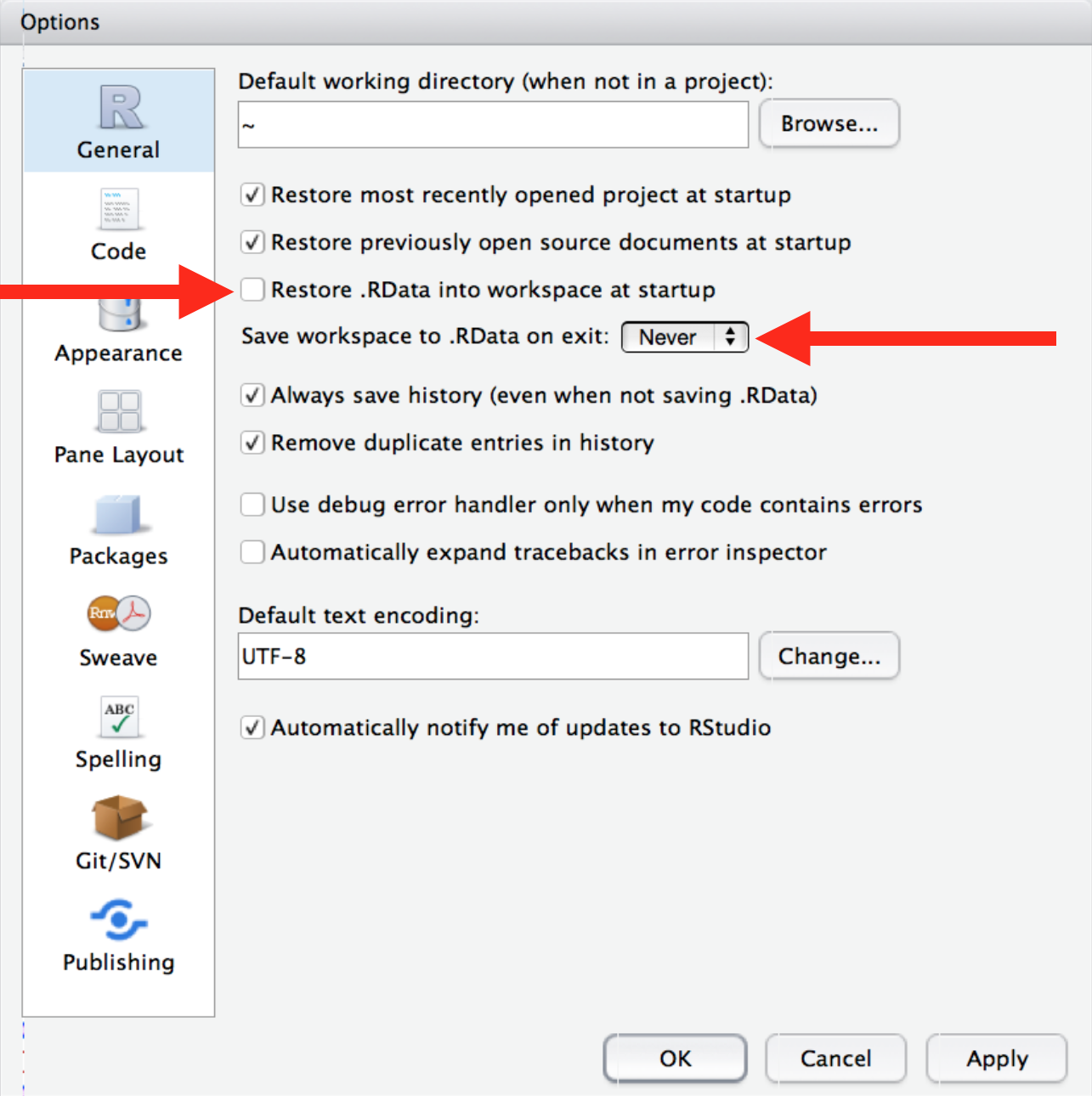
This will cause you some short-term pain, because now when you restart RStudio, it will not remember the results of the code that you ran last time. But this short-term pain will save you long-term agony, because it will force you to capture all important interactions in your scripts.
8.1.2 Working Directories and Paths
Like many programming languages, R has a powerful notion of the working directory. This is where R looks for files that you ask it to load and where it will put any files that you ask it to save.
RStudio shows your current working directory at the top of the console. You can print this out in R code by running getwd():
I do not recommend it, but you can set the working directory from within R:
The command above prints out a path to your working directory. Think of a path as an address. Paths are incredibly important in programming, but they can be a little tricky. Let’s go into a bit more detail.
Absolute Paths
Absolute paths are paths that point to the same place regardless of your current working directory. They always start with the root directory that holds everything else on your computer.
- In Windows, absolute paths start with a drive letter (e.g.,
C:) or two backslashes (e.g.,\\servername). - In Mac/Linux, they start with a slash
/. This is the leading slash in/users/rterman.
Inside the root directory are several other directories, which we call subdirectories. We know that the directory /home/rterman is stored inside /home because /home is the first part of its name. Similarly, we know that /home is stored inside the root directory / because its name begins with /.
Notice that there are two meanings for the / character:
- When it appears at the front of a file or directory name, it refers to the root directory.
- When it appears inside a name, it is just a separator.
Mac/Linux vs. Windows
There are two basic styles of paths: Mac/Linux and Windows. The main difference is how they separate the components of the path. Mac and Linux use slashes (e.g., plots/diamonds.pdf), whereas Windows uses backslashes (e.g., plots\diamonds.pdf).
R can work with either type, no matter what platform you are currently using. Unfortunately, backslashes mean something special to R, and to get a single backslash in the path, you need to type two backslashes! That makes life frustrating, so I recommend always using the Linux/Mac style with forward slashes.
Home Directory
Sometimes you will see a ~ character in a path.
- In Mac/Linux, the
~is a convenient shortcut to your home directory (/users/rterman). - Windows does not really have the notion of a home directory, so it usually points to your documents directory (
C:\DocumentsandSettings\rterman).
Absolute vs. Relative Paths
You should try not to use absolute paths in your scripts, because they hinder sharing: no one else will have exactly the same directory configuration as you. Another way to direct R to something is to give it a relative path.
Relative paths point to something relative to where you are (i.e., relative to your working directory) rather than from the root of the file system. For example, if your current working directory is /home/rterman, then the relative path data/un.csv directs to the full absolute path: /home/rterman/data/un.csv.
8.1.3 R Projects
As a beginning R user, it is OK to let your home directory, documents directory, or any other weird directory on your computer be R’s working directory.
But from this point forward, you should be organizing your projects into dedicated subdirectories containing all the files associated with a project — input data, R scripts, results, figures…
This is such a common practice that RStudio has built-in support for this via projects.
Let’s make a project together. Click File > New Project, then:
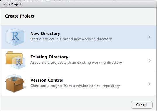
Think carefully about which subdirectory you put the project in. If you do not store it somewhere sensible, it will be hard to find in the future!
Once this process is complete, you will get a new RStudio project. Check that the “home” directory of your project is the current working directory:
Now whenever you refer to a file with a relative path, R will look for the file there.
Go ahead and create a new R script and save it inside the project folder.
Quit RStudio. Inspect the folder associated with your project — notice the .Rproj file. Double-click that file to re-open the project. Notice you get back to where you left off: it is the same working directory and command history, and all the files you were working on are still open. Because you followed my instructions above, however, you will have a completely fresh environment, guaranteeing that you are starting with a clean slate.
8.1.4 File Organization
You should be saving all your files associated with your project in one directory. Here is a basic organization structure that I recommend:
~~~
masters_thesis:
  masters_thesis.Rproj
  01_Clean.R
  02_Model.R
  03_Visualizations.R
  Data/
    raw/
      un-raw.csv
      worldbank-raw.csv
    cleaned/
      country-year.csv
  Results:
    regressions
      h1.txt
      h2.txt
    figures
      bivariate.pdf
      bar_plot.pdf
~~~
Here are some important tips:
- Read raw data from the
Datasubdirectory. Do not ever change or overwrite the raw data! - Export cleaned and altered data into a separate subdirectory.
- Write separate scripts for each stage in the research pipeline. Keep scripts short and focused on one main purpose. If a script gets too long, that might be a sign you need to split it up.
- Write scripts that reproduce your results and figures, which you can save in the
Resultssubdirectory.
8.2 Importing and Exporting
8.2.1 Where Is My Data?
To start, you first need to know where your data lives. Sometimes, the data is stored as a file on your computer, e.g., CSV, Excel, SPSS, or some other file type. When the data is on your computer, we say the data is stored locally.
Data can also be stored externally on the Internet, in a package, or obtained through other sources. For example, some R packages contain datasets (like the gapminder package). Later in this course, we will discuss how to obtain data from web APIs and websites. For now, the rest of the unit discusses data that is stored locally.
8.2.2 Data Storage
Ideally, your data should be stored in a certain file format. I recommend a CSV (comma separated value) file, which formats spreadsheet (rectangular) data in a plain-text format. CSV files are plain-text and can be read into almost any statistical software program, including R. Try to avoid Excel files if you can.
Here are some other tips:
- When working with spreadsheets, the first row is usually reserved for the header, while the first column is used to identify the sampling unit (unique identifier, or key).
- Avoid file names and variable names with blank spaces. This can cause errors when reading in data.
- If you want to concatenate words, insert a
.or_in between two words instead of a space. - Short names are prefered over longer names.
- Try to avoid using names that contain symbols such as
?,$,%,^,&,*,(,),-,#,?,,,<,>,/,|,\,[,],{, and}. - make sure that any missing values in your dataset are indicated with
NAor blank fields (do not use 99 or 77).
8.2.3 Importing Data
Find Paths First
In order to import (or read) data into R, you first have to know where it is and how to find it.
First, remember that you will need to know the current working directory so that you know where R is looking for files. If you are using R Projects, that working directory will be the top-level directory of the project.
Second, you will need to know where the data file is relative to your working directory. If it is stored in the Data/raw/ folder, the relative path to your file will be Data/raw/file-name.csv
Reading Tabular Data
The workhorse for reading into a dataframe is read.table(), which allows any separator (CSV, tab-delimited, etc.). read.csv() is a special case of read.table() for CSV files.
The basic formula is:
# Basic CSV read: Import data with header row, values separated by ",", decimals as "."
mydataset <- read.csv(file="  ", stringsAsFactors=)
Here is a practical example using the PolityIV dataset:
# Import polity
polity <- read.csv("data/polity_sub.csv", stringsAsFactors = F)
head(polity)
#>       country year polity2
#> 1 Afghanistan 1800      -6
#> 2 Afghanistan 1801      -6
#> 3 Afghanistan 1802      -6
#> 4 Afghanistan 1803      -6
#> 5 Afghanistan 1804      -6
#> 6 Afghanistan 1805      -6
We use stringsAsFactors = F in order to treat text columns as character vectors, not as factors. If we do not set this, the default is that all non-numerical columns will be encoded as factors. This behavior usually makes poor sense and is due to historical reasons. At one point in time, factors were faster than character vectors, so R’s read.table() set the default to read in text as factors.
read.table() has a number of other options:
# For importing tabular data with maximum customizability
mydataset <- read.table(file=, header=, sep=, quote=, dec=, fill=, stringsAsFactors=)
You might also see commands like read_csv() (notice the underscore instead of a period). This is the tidyverse version of read.csv() and accomplishes the same task.
Reading Excel Files
Do not use Microsoft Excel files (.xls or .xlsx). But if you must:
# Make sure you have installed the tidyverse suite (only necessary one time)
# install.packages("tidyverse") # Not Run

# Load the "readxl" package (necessary every new R session)
library(readxl)
read_excel() reads both .xls and .xlsx files, and detects the format from the extension.
Here is a real example:
# Example with .xlsx (single sheet)
air <- read_excel("data/airline_small.xlsx", sheet = 1)
air[1:5, 1:5]
#> # A tibble: 5 x 5
#>    Year Month DayofMonth DayOfWeek DepTime
#>   <dbl> <dbl>      <dbl>     <dbl> <chr>
#> 1  2005    11         22         2 1700
#> 2  2008     1         31         4 2216
#> 3  2005     7         17         7 905
#> 4  2008     9         23         2 859
#> 5  2005     3          5         6 827
Reading Stata (.dta) Files
There are many ways to read .dta files into R. I recommend using haven, because it is part of the tidyverse.
For Really Big Data
If you have really big data, read.csv() will be too slow. In these cases, check out the following options:
read_csv()in thereadrpackage is a faster, more helpful drop-in replacement forread.csv()that plays well withtidyversepackages (discussed in future lessons).- The
data.tablepackage is great for reading and manipulating large datasets (orders of gigabytes or 10s of gigabytes).
8.2.4 Exporting Data
You should never go from raw data to results in one script. Typically, you will want to import raw data, clean it, and then export that cleaned dataset onto your computer. That cleaned dataset will then be imported into another script for analysis, in a modular fashion.
To export (or write) data from R onto your computer, you can create individual CSV files or export many data objects into an .RData object.
Writing a csv Spreadsheet
To export an individual dataframe as a spreadsheet, use write.csv()
Let’s write the air dataset as a CSV:
Packaging Data into .RData
Sometimes, it is helpful to write several dataframes at once to be used in later analysis. To do so, we use the save() function to create one file containing many R data objects:
Here is how we can write both air and polity into one file:
We can then read these datasets back into R using load():
Acknowledgements
This page is, in part, derived from the following sources: