Chapter 10 Tidying Data
Even before we conduct analyses or calculations, we need to put our data into the correct format. The goal here is to rearrange a messy dataset into one that is tidy.
The two most important properties of tidy data are:
- Each column is a variable.
- Each row is an observation.
Tidy data is easier to work with because you have a consistent way of referring to variables (as column names) and observations (as row indices). The data then becomes easier to manipulate, visualize, and model.
For more on the concept of tidy data, read Hadley Wickham’s paper here.
10.1 Wide vs. Long Formats
Tidy datasets are all alike, but every messy dataset is messy in its own way.
Hadley Wickham
Tabular datasets can be arranged in many ways. For instance, consider the data below. Each dataset displays information on heart rates observed in individuals across three different time periods, but the data are organized differently in each table.
wide <- data.frame(
  name = c("Wilbur", "Petunia", "Gregory"),
  time1 = c(67, 80, 64),
  time2 = c(56, 90, 50),
  time3 = c(70, 67, 101)
)
wide
#>      name time1 time2 time3
#> 1  Wilbur    67    56    70
#> 2 Petunia    80    90    67
#> 3 Gregory    64    50   101

long <- data.frame(
  name = c("Wilbur", "Petunia", "Gregory", "Wilbur", "Petunia", "Gregory", "Wilbur", "Petunia", "Gregory"),
  time = c(1, 1, 1, 2, 2, 2, 3, 3, 3),
  heartrate = c(67, 80, 64, 56, 90, 50, 70, 67, 10)
)
long
#>      name time heartrate
#> 1  Wilbur    1        67
#> 2 Petunia    1        80
#> 3 Gregory    1        64
#> 4  Wilbur    2        56
#> 5 Petunia    2        90
#> 6 Gregory    2        50
#> 7  Wilbur    3        70
#> 8 Petunia    3        67
#> 9 Gregory    3        10
Question: Which one of these do you think is the tidy format?
Answer: The first dataframe (the “wide” one) would not be considered tidy because values (i.e., heart rate) are spread across multiple columns.
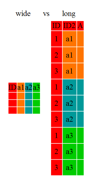
We often refer to these different structures as “long” vs. “wide” formats:
In the “long” format, you usually have one column for the observed variable, and the other columns are ID variables.
In the “wide” format, each row is often a site/subject/patient, and you have multiple observation variables containing the same type of data. These can be either repeated observations over time or observations of multiple variables (or a mix of both). In the case above, we had the same kind of data (heart rate) entered across three different columns, corresponding to three different time periods.
You may find data input in the “wide” format to be simpler, and some other applications may prefer “wide”-format data. However, many of R’s functions have been designed assuming you have “long”-format data.
10.2 Tidying the Gapminder Data
Let’s look at the structure of our original gapminder dataframe:
library(gapminder)

gap <- gapminder
head(gap)
#> # A tibble: 6 x 6
#>   country     continent  year lifeExp      pop gdpPercap
#>   <fct>       <fct>     <int>   <dbl>    <int>     <dbl>
#> 1 Afghanistan Asia       1952    28.8  8425333      779.
#> 2 Afghanistan Asia       1957    30.3  9240934      821.
#> 3 Afghanistan Asia       1962    32.0 10267083      853.
#> 4 Afghanistan Asia       1967    34.0 11537966      836.
#> 5 Afghanistan Asia       1972    36.1 13079460      740.
#> 6 Afghanistan Asia       1977    38.4 14880372      786.
Question: Is this dataframe wide or long?
Answer: This dataframe is somewhere in between the purely ‘long’ and ‘wide’ formats. We have three “ID variables” (continent, country, year) and three “observation variables” (pop, lifeExp, gdpPercap).
Despite not having all observations in one column, this intermediate format makes sense given that all three observation variables have different units. As we have seen, many of the functions in R are often vector-based, and you usually do not want to do mathematical operations on values with different units.
On the other hand, there are some instances in which a purely long or wide format is ideal (e.g., plotting). Likewise, sometimes you will get data on your desk that is poorly organized, and you will need to reshape it.
10.3 tidyr Functions
Thankfully, the tidyr package will help you efficiently transform your data regardless of their original format.
10.3.1 gather
Until now, we have been using the nicely formatted original gapminder dataset. This dataset is not quite wide and not quite long – it is something in the middle – but ‘real’ data (i.e., our own research data) will never be so well organized. Here let’s start with the wide-format version of the gapminder dataset.
gap_wide <- read.csv("data/gapminder_wide.csv", stringsAsFactors = FALSE)
head(gap_wide)
#>   continent      country gdpPercap_1952 gdpPercap_1957 gdpPercap_1962
#> 1    Africa      Algeria           2449           3014           2551
#> 2    Africa       Angola           3521           3828           4269
#> 3    Africa        Benin           1063            960            949
#> 4    Africa     Botswana            851            918            984
#> 5    Africa Burkina Faso            543            617            723
#> 6    Africa      Burundi            339            380            355
#>   gdpPercap_1967 gdpPercap_1972 gdpPercap_1977 gdpPercap_1982 gdpPercap_1987
#> 1           3247           4183           4910           5745           5681
#> 2           5523           5473           3009           2757           2430
#> 3           1036           1086           1029           1278           1226
#> 4           1215           2264           3215           4551           6206
#> 5            795            855            743            807            912
#> 6            413            464            556            560            622
#>   gdpPercap_1992 gdpPercap_1997 gdpPercap_2002 gdpPercap_2007 lifeExp_1952
#> 1           5023           4797           5288           6223         43.1
#> 2           2628           2277           2773           4797         30.0
#> 3           1191           1233           1373           1441         38.2
#> 4           7954           8647          11004          12570         47.6
#> 5            932            946           1038           1217         32.0
#> 6            632            463            446            430         39.0
#>   lifeExp_1957 lifeExp_1962 lifeExp_1967 lifeExp_1972 lifeExp_1977 lifeExp_1982
#> 1         45.7         48.3         51.4         54.5         58.0         61.4
#> 2         32.0         34.0         36.0         37.9         39.5         39.9
#> 3         40.4         42.6         44.9         47.0         49.2         50.9
#> 4         49.6         51.5         53.3         56.0         59.3         61.5
#> 5         34.9         37.8         40.7         43.6         46.1         48.1
#> 6         40.5         42.0         43.5         44.1         45.9         47.5
#>   lifeExp_1987 lifeExp_1992 lifeExp_1997 lifeExp_2002 lifeExp_2007 pop_1952
#> 1         65.8         67.7         69.2         71.0         72.3  9279525
#> 2         39.9         40.6         41.0         41.0         42.7  4232095
#> 3         52.3         53.9         54.8         54.4         56.7  1738315
#> 4         63.6         62.7         52.6         46.6         50.7   442308
#> 5         49.6         50.3         50.3         50.6         52.3  4469979
#> 6         48.2         44.7         45.3         47.4         49.6  2445618
#>   pop_1957 pop_1962 pop_1967 pop_1972 pop_1977 pop_1982 pop_1987 pop_1992
#> 1 10270856 11000948 12760499 14760787 17152804 20033753 23254956 26298373
#> 2  4561361  4826015  5247469  5894858  6162675  7016384  7874230  8735988
#> 3  1925173  2151895  2427334  2761407  3168267  3641603  4243788  4981671
#> 4   474639   512764   553541   619351   781472   970347  1151184  1342614
#> 5  4713416  4919632  5127935  5433886  5889574  6634596  7586551  8878303
#> 6  2667518  2961915  3330989  3529983  3834415  4580410  5126023  5809236
#>   pop_1997 pop_2002 pop_2007
#> 1 29072015 31287142 33333216
#> 2  9875024 10866106 12420476
#> 3  6066080  7026113  8078314
#> 4  1536536  1630347  1639131
#> 5 10352843 12251209 14326203
#> 6  6121610  7021078  8390505
The first step towards getting our nice intermediate data format is to first convert from the wide to the long format.
The function gather() will ‘gather’ the observation variables into a single variable. This is sometimes called “melting” your data, because it melts the table from wide to long. Those data will be melted into two variables: one for the variable names and the other for the variable values.
gap_long <- gap_wide %>%
    gather(obstype_year, obs_values, 3:38)
head(gap_long)
#>   continent      country   obstype_year obs_values
#> 1    Africa      Algeria gdpPercap_1952       2449
#> 2    Africa       Angola gdpPercap_1952       3521
#> 3    Africa        Benin gdpPercap_1952       1063
#> 4    Africa     Botswana gdpPercap_1952        851
#> 5    Africa Burkina Faso gdpPercap_1952        543
#> 6    Africa      Burundi gdpPercap_1952        339
Notice that we put three arguments into the gather() function:
- The name for the new ID variable (
obstype_year). - The name for the new amalgamated observation variable (
obs_value). - The indices of the old observation variables (
3:38, signalling columns 3 through 38) that we want to gather into one variable. Notice that we do not want to melt down columns 1 and 2, as these are considered ID variables.
We can select observation variables using:
- Variable indices.
- Variable names (without quotes).
x:zto select all variables between x and z.-yto exclude y.starts_with(x, ignore.case = TRUE): All names that start withx.ends_with(x, ignore.case = TRUE): All names that end withx.contains(x, ignore.case = TRUE): All names that containx.
See the select() function in dplyr for more options.
For instance, here we do the same thing with (1) the starts_with function and (2) the - operator:
# 1. With the starts_with() function:
gap_long <- gap_wide %>%
    gather(obstype_year, obs_values, starts_with('pop'),
           starts_with('lifeExp'), starts_with('gdpPercap'))
head(gap_long)
#>   continent      country obstype_year obs_values
#> 1    Africa      Algeria     pop_1952    9279525
#> 2    Africa       Angola     pop_1952    4232095
#> 3    Africa        Benin     pop_1952    1738315
#> 4    Africa     Botswana     pop_1952     442308
#> 5    Africa Burkina Faso     pop_1952    4469979
#> 6    Africa      Burundi     pop_1952    2445618

# 2. With the - operator:
gap_long <- gap_wide %>%
  gather(obstype_year, obs_values, -continent, -country)
head(gap_long)
#>   continent      country   obstype_year obs_values
#> 1    Africa      Algeria gdpPercap_1952       2449
#> 2    Africa       Angola gdpPercap_1952       3521
#> 3    Africa        Benin gdpPercap_1952       1063
#> 4    Africa     Botswana gdpPercap_1952        851
#> 5    Africa Burkina Faso gdpPercap_1952        543
#> 6    Africa      Burundi gdpPercap_1952        339
However you choose to do it, notice that the output collapses all of the measured variables into two columns: one containing the new ID variable, the other containing the observation value for that row.
10.3.2 separate
You will notice that, in our long dataset, obstype_year actually contains two pieces of information, the observation type (pop, lifeExp, or gdpPercap) and the year.
We can use the separate() function to split the character strings into multiple variables.
gap_long_sep <- gap_long %>%
  separate(obstype_year, into = c('obs_type','year'), sep = "_") %>%
  mutate(year = as.integer(year))
head(gap_long_sep)
#>   continent      country  obs_type year obs_values
#> 1    Africa      Algeria gdpPercap 1952       2449
#> 2    Africa       Angola gdpPercap 1952       3521
#> 3    Africa        Benin gdpPercap 1952       1063
#> 4    Africa     Botswana gdpPercap 1952        851
#> 5    Africa Burkina Faso gdpPercap 1952        543
#> 6    Africa      Burundi gdpPercap 1952        339
10.3.3 spread
The opposite of gather() is spread(). It spreads our observation variables back out to make a wider table. We can use this function to spread our gap_long() to the original “medium” format.
gap_medium <- gap_long_sep %>%
  spread(obs_type, obs_values)
head(gap_medium)
#>   continent country year gdpPercap lifeExp      pop
#> 1    Africa Algeria 1952      2449    43.1  9279525
#> 2    Africa Algeria 1957      3014    45.7 10270856
#> 3    Africa Algeria 1962      2551    48.3 11000948
#> 4    Africa Algeria 1967      3247    51.4 12760499
#> 5    Africa Algeria 1972      4183    54.5 14760787
#> 6    Africa Algeria 1977      4910    58.0 17152804
All we need is some quick fixes to make this dataset identical to the original gapminder dataset:
gap <- gapminder
head(gap)
#> # A tibble: 6 x 6
#>   country     continent  year lifeExp      pop gdpPercap
#>   <fct>       <fct>     <int>   <dbl>    <int>     <dbl>
#> 1 Afghanistan Asia       1952    28.8  8425333      779.
#> 2 Afghanistan Asia       1957    30.3  9240934      821.
#> 3 Afghanistan Asia       1962    32.0 10267083      853.
#> 4 Afghanistan Asia       1967    34.0 11537966      836.
#> 5 Afghanistan Asia       1972    36.1 13079460      740.
#> 6 Afghanistan Asia       1977    38.4 14880372      786.
# Rearrange columns:
gap_medium <- gap_medium %>%
  select(country, continent, year, lifeExp, pop, gdpPercap)
head(gap_medium)
#>   country continent year lifeExp      pop gdpPercap
#> 1 Algeria    Africa 1952    43.1  9279525      2449
#> 2 Algeria    Africa 1957    45.7 10270856      3014
#> 3 Algeria    Africa 1962    48.3 11000948      2551
#> 4 Algeria    Africa 1967    51.4 12760499      3247
#> 5 Algeria    Africa 1972    54.5 14760787      4183
#> 6 Algeria    Africa 1977    58.0 17152804      4910
# Arrange by country, continent, and year:
gap_medium <- gap_medium %>%
  arrange(country,continent,year)
head(gap_medium)
#>       country continent year lifeExp      pop gdpPercap
#> 1 Afghanistan      Asia 1952    28.8  8425333       779
#> 2 Afghanistan      Asia 1957    30.3  9240934       821
#> 3 Afghanistan      Asia 1962    32.0 10267083       853
#> 4 Afghanistan      Asia 1967    34.0 11537966       836
#> 5 Afghanistan      Asia 1972    36.1 13079460       740
#> 6 Afghanistan      Asia 1977    38.4 14880372       786
What we just told you will become obsolete…
gather and spread are being replaced by pivot_longer and pivot_wider in tidyr 1.0.0, which uses ideas from the cdata package to make reshaping easier to think about. In future classes, we will migrate to those functions.
10.4 Dealing with Missing Data
A common challenge in applying quantitative tools to social science problems is dealing with missing data. You’ll see a variety of ways the creators of data sets designate that a piece of data is missing - for example, NA, -99, or -77 are sometimes used to denote a missing piece of data. We recommend using NA, which has a variety of associated functions that are useful when transforming missing data.
10.4.1 na_if
You can use na_if to replace certain pieces of data with NA. Consider the case where lifeExp values below 35 are missing and simply filled in with “unknown”:
This is problematic for many reasons, including that we cannot perform simple mathematical functions on columns with both number and character values:
mean(gap_medium$lifeExp, na.rm = TRUE)
#> Warning in mean.default(gap_medium$lifeExp, na.rm = TRUE): argument is not
#> numeric or logical: returning NA
#> [1] NA
However, NAs are different in the sense that they can exist in a numeric vector, and therefore you still can perform math functions (R will omit those observations with NA). Below, we replace the “unknown” values with NA, and we can then calculate the mean lifeExp.
10.4.2 Replace NA values with replace_na
Sometimes, you will want to replace all NA values in your data (for instance, maybe you know that the true value of anything coded as NA is actually 30). replace_na is a simple command that will replace all NAs with a new value.
gap_na_replaced <- gap_medium %>%
  mutate(lifeExp = replace_na(lifeExp, 30))

head(gap_na_replaced)
#>       country continent year lifeExp      pop gdpPercap
#> 1 Afghanistan      Asia 1952    30.0  8425333       779
#> 2 Afghanistan      Asia 1957    30.0  9240934       821
#> 3 Afghanistan      Asia 1962    30.0 10267083       853
#> 4 Afghanistan      Asia 1967    30.0 11537966       836
#> 5 Afghanistan      Asia 1972    36.1 13079460       740
#> 6 Afghanistan      Asia 1977    38.4 14880372       786
10.5 More tidyverse
dplyr and tidyr have many more functions to help you wrangle and manipulate
your data. See the Data Wrangling Cheatsheet for more.
There are some other useful packages in the tidyverse:
ggplot2for plotting (we will cover this in the Visualization module).readrandhavenfor reading in data.purrrfor working iterations.stringr,lubridate, andforcatsfor manipulating strings, dates, and factors, respectively.- Many many more! Take a peak at the tidyverse GitHub page…
10.6 Challenges
Challenge 1.
Subset the results from Challenge #3 (of the previous chapter) to select only the country, year, and gdpPercap_diff columns. Use tidyr to put it in wide format so that countries are rows and years are columns.
Challenge 2.
Now turn the dataframe above back into the long format with three columns: country, year, and gdpPercap_diff.
Acknowledgments
Some of the materials in this module were adapted from: